2  Supplementary information

2.1 Setup

Code

# Load packages
library(papaja)
library(here)
library(scales)
library(tidyverse)
library(furrr)
library(metafor)
library(brms)
library(tidybayes)
library(cowplot)

# Load custom helper functions
source(here("misc", "helper_functions.R"))

# Read work space from the main text script
load(here("results", "workspace.RData"))

2.2 Supplementary methods

2.2.1 Correlation between dependent samples

Empirical estimate for the correlation (Supplementary Methods 1)

Code

# Compute empirical estimate of the correlation between dependent samples
ri_empirical <- dat_meta %>%
  mutate(
    # Get effect size from paired samples t-test, one sample t-test, or ANOVA
    d_diff = case_when(
      !is.na(d) ~ d,
      !is.na(d_z_t) ~ d_z_t,
      !is.na(d_z_f) ~ d_z_f,
      !is.na(d_z_diff) ~ d_z_diff
    ),
    # Compute empirical correlation
    # Based on the SD of the difference and the SDs within the two conditions
    sd_diff = mean_diff / d_diff,
    ri = (sd_diff^2 - sd_novel^2 - sd_familiar^2) /
      (-2 * sd_novel * sd_familiar)
  ) %>%
  pull(ri)

# Subset articles that have an empirical estimate for the correlation
dat_ri_empirical <- filter(dat_meta, !is.na(ri_empirical))

# Summarise the estimated correlations
list(
  mean = mean(ri_empirical, na.rm = TRUE),
  median = median(ri_empirical, na.rm = TRUE),
  min = min(ri_empirical, na.rm = TRUE),
  max = max(ri_empirical, na.rm = TRUE)
) %>%
  map(print_num)

$mean
[1] "0.58"

$median
[1] "0.59"

$min
[1] "0.03"

$max
[1] "1.00"

2.3 Supplementary tables

2.3.1 Frequentist meta-analyses and meta-regression

Frequentist meta-analysis of mental rotation performance

Code

# Compute frequentist three-level model for the meta-analysis of rotation
res_freq_meta <- rma.mv(
  gi, vi,
  random = ~ 1 | article / experiment,
  data = dat_meta,
  slab = experiment
)
print(res_freq_meta)

Multivariate Meta-Analysis Model (k = 62; method: REML)

Variance Components:

            estim    sqrt  nlvls  fixed              factor 
sigma^2.1  0.0521  0.2283     21     no             article 
sigma^2.2  0.1343  0.3665     62     no  article/experiment 

Test for Heterogeneity:
Q(df = 61) = 257.4619, p-val < .0001

Model Results:

estimate      se    zval    pval   ci.lb   ci.ub 
  0.2102  0.0773  2.7209  0.0065  0.0588  0.3617  ** 

---
Signif. codes:  0 '***' 0.001 '**' 0.01 '*' 0.05 '.' 0.1 ' ' 1

Variance at each level of the model

Code

# Check share of variance at each level of the model
round(res_freq_meta$sigma2[1] / sum(res_freq_meta$sigma2), 3)
round(res_freq_meta$sigma2[2] / sum(res_freq_meta$sigma2), 3)

[1] 0.28
[1] 0.72

Frequentist meta-regression of mental rotation performance

Code

# Compute frequentist meta-regression with gender, age, and task
res_freq_reg <- rma.mv(
  gi, vi,
  mods = ~ gender * age_c + task,
  random = ~ 1 | article / experiment,
  data = dat_meta,
  slab = experiment
)
print(res_freq_reg)

Multivariate Meta-Analysis Model (k = 62; method: REML)

Variance Components:

            estim    sqrt  nlvls  fixed              factor 
sigma^2.1  0.0348  0.1866     21     no             article 
sigma^2.2  0.1217  0.3489     62     no  article/experiment 

Test for Residual Heterogeneity:
QE(df = 55) = 198.8077, p-val < .0001

Test of Moderators (coefficients 2:7):
QM(df = 6) = 13.6854, p-val = 0.0334

Model Results:

                 estimate      se    zval    pval    ci.lb   ci.ub 
intrcpt            0.3903  0.1097  3.5581  0.0004   0.1753  0.6052  *** 
gender2-1          0.0265  0.2156  0.1229  0.9022  -0.3961  0.4492      
gender3-2          0.4007  0.1884  2.1272  0.0334   0.0315  0.7699    * 
age_c              0.5981  0.3807  1.5711  0.1162  -0.1481  1.3443      
task2-1            0.4419  0.1951  2.2651  0.0235   0.0595  0.8243    * 
gender2-1:age_c    0.3789  0.8243  0.4597  0.6457  -1.2367  1.9946      
gender3-2:age_c    0.5745  0.9221  0.6231  0.5332  -1.2327  2.3818      

---
Signif. codes:  0 '***' 0.001 '**' 0.01 '*' 0.05 '.' 0.1 ' ' 1

Frequentist meta-analysis of gender differences

Code

# Compute frequentist three-level model for the meta-analysis of gender
res_freq_gender <- rma.mv(
  gi, vi,
  random = ~ 1 | article / experiment,
  data = dat_gender,
  slab = experiment
)
print(res_freq_gender)

Multivariate Meta-Analysis Model (k = 30; method: REML)

Variance Components:

            estim    sqrt  nlvls  fixed              factor 
sigma^2.1  0.0463  0.2153     19     no             article 
sigma^2.2  0.0048  0.0695     30     no  article/experiment 

Test for Heterogeneity:
Q(df = 29) = 38.9840, p-val = 0.1020

Model Results:

estimate      se    zval    pval    ci.lb   ci.ub 
  0.1461  0.0795  1.8373  0.0662  -0.0098  0.3020  . 

---
Signif. codes:  0 '***' 0.001 '**' 0.01 '*' 0.05 '.' 0.1 ' ' 1

Summary table (Supplementary Table 1)

Code

# Format all frequentist results together as a table
tabs2 <- map2_dfr(
  list(res_freq_meta, res_freq_reg, res_freq_gender),
  c(
    "Meta-analysis of mental rotation",
    "Meta-regression of mental rotation",
    "Meta-analysis of gender differences"
  ),
  ~ print_res_freq_table(
    res_freq = .x, label_1 = .y, label_col_1 = "Model",
    print_sigma2s = TRUE
  )
) %>%
  # Rename parameter labels
  mutate(
    Parameter = c(
      "Hedges' $g$",
      "$\\sigma_{\\text{article}}^2$",
      "$\\sigma_{\\text{experiment}}^2$",
      "Intercept (Hedges' $g$)",
      "Female - mixed",
      "Male - female",
      "Age (per year)",
      "Habituation - VoE",
      "(Female - mixed) $\\times$ age",
      "(Male - female) $\\times$ age",
      "$\\sigma_{\\text{article}}^2$",
      "$\\sigma_{\\text{experiment}}^2$",
      "Hedges' $g$",
      "$\\sigma_{\\text{article}}^2$",
      "$\\sigma_{\\text{experiment}}^2$"
    )
  ) %>%
  # Replace NAs with blank cells
  mutate(across(.fns = ~ ifelse(is.na(.), "", .)))

# Save the table
write_tsv(tabs2, file = here(tables_dir, "tabs2_frequentist.tsv"))

# Add footnotes
colnames(tabs2)[4] <- str_c(colnames(tabs2)[4], "^a^")
colnames(tabs2)[7] <- str_c(colnames(tabs2)[7], "^b^")

# Display the table
apa_table(
  tabs2,
  note = str_c(
    "^a^ = standard error, ",
    "^b^ = 95\\% confidence interval."
  ),
  font_size = "scriptsize",
  escape = FALSE,
  align = "llrrrrr"
)

(#tab:unnamed-chunk-14)

**

Model	Parameter	Estimate	\(SE\)a	\(z\)	\(p\)	95% CIb
Meta-analysis of mental rotation	Hedges’ \(g\)	0.21	0.08	2.72	0.007	[0.06, 0.36]
	\(\sigma_{\text{article}}^2\)	0.05
	\(\sigma_{\text{experiment}}^2\)	0.13
Meta-regression of mental rotation	Intercept (Hedges’ \(g\))	0.39	0.11	3.56	< 0.001	[0.18, 0.61]
	Female - mixed	0.03	0.22	0.12	0.902	[-0.40, 0.45]
	Male - female	0.40	0.19	2.13	0.033	[0.03, 0.77]
	Age (per year)	0.60	0.38	1.57	0.116	[-0.15, 1.34]
	Habituation - VoE	0.44	0.20	2.27	0.024	[0.06, 0.82]
	(Female - mixed) \(\times\) age	0.38	0.82	0.46	0.646	[-1.24, 1.99]
	(Male - female) \(\times\) age	0.57	0.92	0.62	0.533	[-1.23, 2.38]
	\(\sigma_{\text{article}}^2\)	0.03
	\(\sigma_{\text{experiment}}^2\)	0.12
Meta-analysis of gender differences	Hedges’ \(g\)	0.15	0.08	1.84	0.066	[-0.01, 0.30]
	\(\sigma_{\text{article}}^2\)	0.05
	\(\sigma_{\text{experiment}}^2\)	0.00

Note. ^a = standard error, ^b = 95% confidence interval.

 

2.3.2 Jackknife (leave-one-out) analysis

Re-fit Bayesian meta-analysis, leaving one experiment out

Code

# Re-run the jackknife analysis if requested
if (run$jackknife_analysis) {
  # Re-fit the meta-analysis, leaving out one experiment at a time
  # Using parallelization with `furrr`
  n_cores <- availableCores()
  n_workers <- n_cores %/% n_chains
  plan(multisession, workers = n_workers)
  tabs3 <- future_map_dfr(seq_len(nrow(dat_meta)), function(jackknife_index) {
    dat_jackknife <- dat_meta[-jackknife_index, ]
    res_jackknife <- update(
      res_meta,
      newdata = dat_jackknife,
      seed = seed,
      refresh = 0
    )
    print_res_table(
      res_jackknife,
      label_1 = dat_meta$article[jackknife_index],
      label_2 = dat_meta$group[jackknife_index],
      label_col_1 = "Article", label_col_2 = "Left-out experiment"
    )
  }) %>%
    # Show article labels only for the first experiment (row) per article
    mutate(
      Article = if_else(Article == lag(Article, default = ""), "", Article),
    )

  # Save the table
  write_tsv(tabs3, file = here(tables_dir, "tabs3_jackknife.tsv"))
}

Summary table (Supplementary Table 3)

Code

# Read jackknife table from file
tabs3 <- read_tsv(
  here(tables_dir, "tabs3_jackknife.tsv"),
  col_types = "c", na = character()
)

# Add footnotes
colnames(tabs3)[6] <- str_c(colnames(tabs3)[6], "^a^")

# Display the table
apa_table(
  tabs3,
  font_size = "scriptsize",
  note = "^a^ = intraclass correlation.",
  landscape = TRUE, escape = FALSE, align = "llrrrr"
)

(#tab:unnamed-chunk-18)

**

Article	Left-out experiment	Hedges’ \(g\)	\(\sigma_\text{article}^2\)	\(\sigma_\text{experiment}^2\)	\({ICC}\)a
Rochat & Hespos 1996	Experiment 1	0.20 [0.05, 0.37]	0.05 [0.00, 0.17]	0.15 [0.07, 0.27]	0.25 [0.00, 0.63]
Hespos & Rochat 1997	Experiment 2	0.20 [0.05, 0.36]	0.04 [0.00, 0.16]	0.15 [0.07, 0.27]	0.21 [0.00, 0.60]
	Experiment 3	0.20 [0.05, 0.36]	0.05 [0.00, 0.16]	0.15 [0.07, 0.27]	0.22 [0.00, 0.61]
	Experiment 4, 4-months-old infants	0.21 [0.06, 0.37]	0.06 [0.00, 0.18]	0.15 [0.07, 0.27]	0.27 [0.00, 0.65]
	Experiment 4, 6-months-old infants	0.20 [0.06, 0.35]	0.05 [0.00, 0.16]	0.15 [0.07, 0.27]	0.22 [0.00, 0.61]
	Experiment 5, 6-months-old infants	0.20 [0.05, 0.36]	0.05 [0.00, 0.16]	0.15 [0.07, 0.27]	0.22 [0.00, 0.61]
	Experiment 6, 6-months-old infants	0.20 [0.05, 0.35]	0.04 [0.00, 0.16]	0.15 [0.07, 0.27]	0.22 [0.00, 0.61]
Moore & Johnson 2008	Females	0.22 [0.06, 0.38]	0.06 [0.00, 0.18]	0.15 [0.06, 0.27]	0.27 [0.00, 0.65]
	Males	0.20 [0.04, 0.36]	0.05 [0.00, 0.17]	0.15 [0.06, 0.26]	0.26 [0.00, 0.64]
Quinn & Liben 2008	Females	0.22 [0.06, 0.39]	0.07 [0.00, 0.22]	0.14 [0.06, 0.26]	0.32 [0.00, 0.72]
	Males	0.18 [0.04, 0.34]	0.05 [0.00, 0.16]	0.12 [0.05, 0.23]	0.28 [0.00, 0.66]
Moore & Johnson 2011	Females	0.20 [0.05, 0.36]	0.05 [0.00, 0.18]	0.15 [0.07, 0.27]	0.26 [0.00, 0.65]
	Males	0.22 [0.07, 0.38]	0.05 [0.00, 0.16]	0.14 [0.06, 0.25]	0.26 [0.00, 0.64]
Frick & Möhring 2013	10-months-old infants	0.19 [0.04, 0.35]	0.05 [0.00, 0.17]	0.14 [0.06, 0.25]	0.26 [0.00, 0.65]
	8-months-old infants	0.21 [0.06, 0.38]	0.06 [0.00, 0.18]	0.15 [0.06, 0.27]	0.27 [0.00, 0.66]
Möhring & Frick 2013	Exploration group	0.20 [0.05, 0.36]	0.05 [0.00, 0.17]	0.15 [0.07, 0.27]	0.25 [0.00, 0.64]
	Observation group	0.21 [0.06, 0.37]	0.05 [0.00, 0.17]	0.15 [0.07, 0.27]	0.25 [0.00, 0.63]
Schwarzer et al. 2013a	Crawling infants	0.20 [0.04, 0.36]	0.06 [0.00, 0.18]	0.15 [0.06, 0.26]	0.27 [0.00, 0.66]
	Non-crawling infants	0.22 [0.06, 0.38]	0.06 [0.00, 0.18]	0.14 [0.06, 0.26]	0.27 [0.00, 0.66]
Schwarzer et al. 2013b	Crawling infants	0.20 [0.04, 0.35]	0.05 [0.00, 0.17]	0.15 [0.06, 0.26]	0.26 [0.00, 0.64]
	Non-crawling infants	0.21 [0.06, 0.38]	0.06 [0.00, 0.18]	0.15 [0.07, 0.27]	0.26 [0.00, 0.65]
Frick & Wang 2014	Experiment 1, 14-months-old infants	0.22 [0.06, 0.38]	0.06 [0.00, 0.18]	0.14 [0.06, 0.25]	0.30 [0.00, 0.67]
	Experiment 1, 16-months-old infants	0.20 [0.05, 0.36]	0.05 [0.00, 0.16]	0.15 [0.07, 0.26]	0.25 [0.00, 0.63]
	Experiment 2, 14-months-old infants	0.21 [0.05, 0.37]	0.05 [0.00, 0.16]	0.15 [0.07, 0.27]	0.24 [0.00, 0.61]
	Experiment 2, 16-months-old infants	0.20 [0.05, 0.37]	0.05 [0.00, 0.17]	0.15 [0.07, 0.26]	0.25 [0.00, 0.63]
	Experiment 3, other-turning group	0.21 [0.06, 0.37]	0.05 [0.00, 0.17]	0.15 [0.07, 0.26]	0.26 [0.00, 0.63]
	Experiment 3, self-turning group	0.20 [0.05, 0.36]	0.05 [0.00, 0.16]	0.15 [0.07, 0.26]	0.25 [0.00, 0.63]
Quinn & Liben 2014	Experiment 2, 6-months-old females	0.22 [0.06, 0.38]	0.06 [0.00, 0.19]	0.14 [0.06, 0.26]	0.29 [0.00, 0.67]
	Experiment 2, 6-months-old males	0.19 [0.04, 0.35]	0.05 [0.00, 0.16]	0.14 [0.06, 0.25]	0.25 [0.00, 0.64]
	Experiment 2, 9-months-old females	0.21 [0.06, 0.37]	0.06 [0.00, 0.18]	0.15 [0.06, 0.26]	0.27 [0.00, 0.65]
	Experiment 2, 9-months-old males	0.20 [0.05, 0.35]	0.05 [0.00, 0.16]	0.14 [0.06, 0.26]	0.24 [0.00, 0.63]
Lauer et al. 2015	Females	0.20 [0.05, 0.37]	0.05 [0.00, 0.17]	0.15 [0.07, 0.27]	0.23 [0.00, 0.63]
	Males	0.19 [0.04, 0.34]	0.04 [0.00, 0.14]	0.14 [0.06, 0.25]	0.21 [0.00, 0.59]
Antrilli & Wang 2016	Vertical-stripes group	0.19 [0.04, 0.34]	0.05 [0.00, 0.15]	0.14 [0.06, 0.26]	0.24 [0.00, 0.62]
Christodoulou et al. 2016	Females	0.21 [0.06, 0.37]	0.05 [0.00, 0.16]	0.15 [0.07, 0.27]	0.22 [0.00, 0.61]
	Males	0.22 [0.08, 0.37]	0.04 [0.00, 0.14]	0.14 [0.06, 0.25]	0.21 [0.00, 0.58]
Constantinescu et al. 2018	Females	0.22 [0.06, 0.39]	0.06 [0.00, 0.19]	0.14 [0.06, 0.25]	0.31 [0.00, 0.70]
	Males	0.19 [0.04, 0.35]	0.06 [0.00, 0.18]	0.13 [0.06, 0.25]	0.29 [0.00, 0.68]
Erdmann et al. 2018	5-months-old females	0.21 [0.06, 0.38]	0.05 [0.00, 0.17]	0.15 [0.07, 0.27]	0.23 [0.00, 0.62]
	5-months-old males	0.21 [0.06, 0.37]	0.05 [0.00, 0.16]	0.15 [0.07, 0.27]	0.22 [0.00, 0.60]
	9-months-old females	0.21 [0.06, 0.36]	0.05 [0.00, 0.16]	0.16 [0.07, 0.28]	0.23 [0.00, 0.61]
	9-months-old males	0.21 [0.06, 0.37]	0.05 [0.00, 0.16]	0.15 [0.07, 0.28]	0.23 [0.00, 0.61]
Gerhard & Schwarzer 2018	Crawling infants, 0° group	0.20 [0.04, 0.37]	0.06 [0.00, 0.18]	0.14 [0.06, 0.26]	0.28 [0.00, 0.66]
	Crawling infants, 54° group	0.22 [0.07, 0.37]	0.05 [0.00, 0.16]	0.14 [0.06, 0.26]	0.25 [0.00, 0.63]
	Non-crawling infants, 0° group	0.21 [0.06, 0.37]	0.05 [0.00, 0.16]	0.15 [0.07, 0.27]	0.23 [0.00, 0.61]
	Non-crawling infants, 54° group	0.21 [0.05, 0.36]	0.05 [0.00, 0.16]	0.15 [0.07, 0.27]	0.24 [0.00, 0.62]
Slone et al. 2018	Mittens-first group, females	0.21 [0.05, 0.37]	0.05 [0.00, 0.17]	0.15 [0.07, 0.27]	0.24 [0.00, 0.62]
	Mittens-first group, males	0.21 [0.05, 0.37]	0.05 [0.00, 0.17]	0.15 [0.07, 0.27]	0.24 [0.00, 0.62]
	Mittens-second group, females	0.22 [0.06, 0.37]	0.05 [0.00, 0.16]	0.15 [0.07, 0.26]	0.24 [0.00, 0.62]
	Mittens-second group, males	0.21 [0.06, 0.36]	0.05 [0.00, 0.16]	0.15 [0.07, 0.27]	0.24 [0.00, 0.62]
Kaaz & Heil 2020	Experiment 1, females	0.21 [0.06, 0.37]	0.05 [0.00, 0.16]	0.15 [0.07, 0.27]	0.23 [0.00, 0.61]
	Experiment 1, males	0.21 [0.06, 0.37]	0.05 [0.00, 0.17]	0.15 [0.07, 0.27]	0.24 [0.00, 0.62]
	Experiment 2, females	0.21 [0.06, 0.37]	0.05 [0.00, 0.16]	0.15 [0.07, 0.27]	0.23 [0.00, 0.60]
	Experiment 2, males	0.20 [0.05, 0.36]	0.05 [0.00, 0.17]	0.15 [0.07, 0.27]	0.26 [0.00, 0.64]
Gerhard-Samunda et al. 2021	Horizontal-stripes group, crawling infants	0.22 [0.06, 0.38]	0.05 [0.00, 0.17]	0.14 [0.06, 0.25]	0.27 [0.00, 0.65]
	Horizontal-stripes group, non-crawling infants	0.21 [0.06, 0.37]	0.05 [0.00, 0.17]	0.15 [0.07, 0.27]	0.25 [0.00, 0.62]
	Vertical-stripes group, crawling infants	0.20 [0.05, 0.36]	0.06 [0.00, 0.18]	0.14 [0.06, 0.26]	0.28 [0.00, 0.65]
	Vertical-stripes group, non-crawling infants	0.21 [0.06, 0.37]	0.05 [0.00, 0.16]	0.15 [0.07, 0.27]	0.25 [0.00, 0.62]
Kelch et al. 2021	Experiment 1, crawling infants	0.22 [0.07, 0.37]	0.05 [0.00, 0.16]	0.14 [0.06, 0.25]	0.24 [0.00, 0.63]
	Experiment 1, non-crawling infants	0.21 [0.06, 0.36]	0.05 [0.00, 0.16]	0.15 [0.07, 0.27]	0.24 [0.00, 0.62]
	Experiment 2, crawling infants	0.21 [0.06, 0.37]	0.05 [0.00, 0.16]	0.15 [0.07, 0.27]	0.23 [0.00, 0.61]
	Experiment 2, non-crawling infants	0.21 [0.05, 0.37]	0.06 [0.00, 0.18]	0.15 [0.07, 0.27]	0.26 [0.00, 0.64]

Note. ^a = intraclass correlation.

 

2.3.3 PRISMA checklist

Print PRISMA checklist (Supplementary Table 4)

Code

# Read PRISMA checklist from file
tabs4 <- read_tsv(here(data_dir, "05_prisma.tsv"), na = character())

# Display the table
apa_table(
  tabs4,
  font_size = "scriptsize",
  landscape = TRUE,
  align = "lllll" # For Word
  # align = "p{1.5cm}p{2.5cm}p{1cm}p{12cm}p{5.5cm}" # For LaTeX
)

(#tab:unnamed-chunk-20)

**

Section	Topic	Item #	Checklist item	Location where item is reported
Title	Title	1	Identify the report as a systematic review.	–
Abstract	Abstract	2	See the PRISMA 2020 for Abstracts checklist.	Abstract
Introduction	Rationale	3	Describe the rationale for the review in the context of existing knowledge.	Introduction
	Objectives	4	Provide an explicit statement of the objective(s) or question(s) the review addresses.	Introduction
Methods	Eligibility criteria	5	Specify the inclusion and exclusion criteria for the review and how studies were grouped for the syntheses.	Methods: Eligibility criteria
	Information sources	6	Specify all databases, registers, websites, organisations, reference lists and other sources searched or consulted to identify studies. Specify the date when each source was last searched or consulted.	Methods: Information sources and search strategy
	Search strategy	7	Present the full search strategies for all databases, registers and websites, including any filters and limits used.	Methods: Information sources and search strategy
	Selection process	8	Specify the methods used to decide whether a study met the inclusion criteria of the review, including how many reviewers screened each record and each report retrieved, whether they worked independently, and if applicable, details of automation tools used in the process.	Methods: Selection process
	Data collection process	9	Specify the methods used to collect data from reports, including how many reviewers collected data from each report, whether they worked independently, any processes for obtaining or confirming data from study investigators, and if applicable, details of automation tools used in the process.	Methods: Data collection process and items
	Data items	10a	List and define all outcomes for which data were sought. Specify whether all results that were compatible with each outcome domain in each study were sought (e.g. for all measures, time points, analyses), and if not, the methods used to decide which results to collect.	Methods: Data collection process and items
		10b	List and define all other variables for which data were sought (e.g. participant and intervention characteristics, funding sources). Describe any assumptions made about any missing or unclear information.	Methods: Data collection process and items
	Study risk of bias assessment	11	Specify the methods used to assess risk of bias in the included studies, including details of the tool(s) used, how many reviewers assessed each study and whether they worked independently, and if applicable, details of automation tools used in the process.	Methods: Selection process
	Effect measures	12	Specify for each outcome the effect measure(s) (e.g. risk ratio, mean difference) used in the synthesis or presentation of results.	Methods: Effect measures
	Synthesis methods	13a	Describe the processes used to decide which studies were eligible for each synthesis (e.g. tabulating the study intervention characteristics and comparing against the planned groups for each synthesis (item #5)).	Methods: Data collection process and items
		13b	Describe any methods required to prepare the data for presentation or synthesis, such as handling of missing summary statistics, or data conversions.	Methods: Effect measures
		13c	Describe any methods used to tabulate or visually display results of individual studies and syntheses.	Results: Figure 1
		13d	Describe any methods used to synthesize results and provide a rationale for the choice(s). If meta-analysis was performed, describe the model(s), method(s) to identify the presence and extent of statistical heterogeneity, and software package(s) used.	Methods: Bayesian meta-analysis; Methods: Frequentist meta-analysis
		13e	Describe any methods used to explore possible causes of heterogeneity among study results (e.g. subgroup analysis, meta-regression).	Methods: Bayesian meta-regression
		13f	Describe any sensitivity analyses conducted to assess robustness of the synthesized results.	Methods: Bayesian meta-analysis; Supplementary Methods 1
	Reporting bias assessment	14	Describe any methods used to assess risk of bias due to missing results in a synthesis (arising from reporting biases).	Methods: Publication bias asssessment
	Certainty assessment	15	Describe any methods used to assess certainty (or confidence) in the body of evidence for an outcome.	Methods: Publication bias asssessment
Results	Study selection	16a	Describe the results of the search and selection process, from the number of records identified in the search to the number of studies included in the review, ideally using a flow diagram.	Introduction; Results: Mental rotation performance; Supplementary Figure 2
		16b	Cite studies that might appear to meet the inclusion criteria, but which were excluded, and explain why they were excluded.	Methods: Selection process
	Study characteristics	17	Cite each included study and present its characteristics.	Supplementary Table 1
	Risk of bias in studies	18	Present assessments of risk of bias for each included study.	–
	Results of individual studies	19	For all outcomes, present, for each study: (a) summary statistics for each group (where appropriate) and (b) an effect estimate and its precision (e.g. confidence/credible interval), ideally using structured tables or plots.	Results: Figure 1
	Results of syntheses	20a	For each synthesis, briefly summarise the characteristics and risk of bias among contributing studies.	Introduction
		20b	Present results of all statistical syntheses conducted. If meta-analysis was done, present for each the summary estimate and its precision (e.g. confidence/credible interval) and measures of statistical heterogeneity. If comparing groups, describe the direction of the effect.	Results: Mental rotation performance
		20c	Present results of all investigations of possible causes of heterogeneity among study results.	Results: Effects of gender, age, and task
		20d	Present results of all sensitivity analyses conducted to assess the robustness of the synthesized results.	Supplementary Tables 7, 8, and 9
	Reporting biases	21	Present assessments of risk of bias due to missing results (arising from reporting biases) for each synthesis assessed.	Results: Publication bias assessment; Supplementary Methods 2; Supplementary Tables 3, 10 and 11
	Certainty of evidence	22	Present assessments of certainty (or confidence) in the body of evidence for each outcome assessed.	Results: Figure 1; Results: Figure 2
Discussion	Discussion	23a	Provide a general interpretation of the results in the context of other evidence.	Discussion
		23b	Discuss any limitations of the evidence included in the review.	Discussion
		23c	Discuss any limitations of the review processes used.	Discussion
		23d	Discuss implications of the results for practice, policy, and future research.	Discussion
Other information	Registration and protocol	24a	Provide registration information for the review, including register name and registration number, or state that the review was not registered.	–
		24b	Indicate where the review protocol can be accessed, or state that a protocol was not prepared.	–
		24c	Describe and explain any amendments to information provided at registration or in the protocol.	–
	Support	25	Describe sources of financial or non-financial support for the review, and the role of the funders or sponsors in the review.	–
	Competing interests	26	Declare any competing interests of review authors.	Competing interests
	Availability of data, code and other materials	27	Report which of the following are publicly available and where they can be found: template data collection forms; data extracted from included studies; data used for all analyses; analytic code; any other materials used in the review.	Methods: Data availability; Methods: Code availability

2.3.4 Effect size conversion

Formulas for mental rotation performance (Supplementary Table 5)

=

Available statistics	Conversion to standardized mean difference (Hedges’ \(g\))
(1) Cohen’s \(d\) and sample size (Goulet-Pelletier and Cousineau 2018; Hedges and Olkin 1985)	\({df}=2(n-1)\); \(J({df})=\frac{\Gamma(\frac{1}{2}{df})}{\sqrt{\frac{{df}}{2}}\Gamma(\frac{1}{2}({df}-1))}\); \(g_\text{rotation}=d\cdot{J}({df})\)
(2) \(t\) statistic and sample size (Rosenthal 1991)	\(d=\frac{t}{\sqrt{n}}\);then (1)
(3) \(F\) statistic and sample size (Lakens 2013)	\(t=\sqrt{F}\);then (2)
(4) Mean difference between conditions (Lakens 2013)	\(d=\frac{m_\text{diff}}{{SD}_\text{diff}}\);then (1)
(5) Mean looking times$ per condition (Cumming 2012)	\({SD}_\text{av}=\sqrt{\frac{{SD}_\text{novel}^2+{SD}_\text{familiar}^2}{2}}\); \(d=\frac{m_\text{novel}-m_\text{familiar}}{{SD}_\text{av}}\);then (1)
(6) Mean novelty preference score (Lakens 2013)	\(d=\frac{m_\text{pref}}{{SD}_\text{pref}}\);then (1)

Formulas for gender differences (Supplementary Table 6)

Available statistics	Conversion to standardized mean difference (Hedges’ \(g\))
(1) Cohen’s \(d\) and group sizes (Goulet-Pelletier and Cousineau 2018; Hedges and Olkin 1985)	\({df}=n_\text{female}+n_\text{male}-2\); \(J({df})=\frac{\Gamma(\frac{1}{2}{df})}{\sqrt{\frac{{df}}{2}}\Gamma(\frac{1}{2}({df}-1))}\); \(g_\text{gender}=d\cdot{J({df})}\)
(2) \(t\) statistic and group sizes (Lakens 2013)	\(d=t\sqrt{\frac{1}{n_\text{female}}+\frac{1}{n_\text{male}}}\);then (1)
(3) \(F\) statistic and group sizes (Lakens 2013)	\(t=\sqrt{F}\);then (2)
(4) Mean differences between conditions or preference scores (Lakens 2013)	\({SD}_\text{pooled}=\sqrt{\frac{(n_\text{female}-1){SD}_\text{female}^2 +(n_\text{male}-1){SD}_\text{male}^2}{df}}\); \(d=\frac{m_\text{female}-m_\text{male}}{{SD}_\text{pooled}}\);then (1)

2.3.5 Sensitivity analyses

Re-fit Bayesian meta-analysis with different correlations and priors

Code

# Re-run the sensitivity analyses if requested
if (run$sensitivity_analysis) {
  # Re-run the meta-analysis for different values of r_assumed
  sens_ri <- seq(-0.9, 0.9, by = 0.3) %>%
    map_dfr(function(ri_sens) {
      # Re-compute standard errors of the effect sizes
      dat_ri_sens <- mutate(
        dat_meta,
        vi = (dfi / (dfi - 2)) * ((2 * (1 - ri_sens)) / ni) *
          (1 + gi^2 * (ni / (2 * (1 - ri_sens)))) - (gi^2 / ji^2),
        sei = sqrt(vi)
      )

      # Re-run meta-analysis of mental rotation performance
      res_meta <- update(
        res_meta,
        newdata = dat_ri_sens,
        seed = seed,
        refresh = 0
      )

      # Re-run meta-regression of mental rotation performance
      res_reg <- update(
        res_reg,
        newdata = dat_ri_sens,
        seed = seed,
        refresh = 0
      )

      # Return both as a tibble and add a label
      return(
        tibble(
          manipulation_value = str_c("$r$ = ", print_num(ri_sens)),
          res_meta = list(res_meta),
          res_reg = list(res_reg),
        )
      )
    }) %>%
    bind_cols(
      manipulation_name = c("Assumed correlation", rep("", nrow(.) - 1)), .
    )

  # Prior sensitivity analysis
  sens_prior <- list(
    # Less informative prior for the intercept
    `$b\\sim\\mathcal{U}(-10,10)$` = c(
      set_prior("uniform(-10, 10)", class = "b", coef = "Intercept"),
      set_prior("normal(0, 0.5)", class = "b"),
      set_prior("cauchy(0, 0.3)", class = "sd")
    ),
    # More informative prior for the intercept
    `$b\\sim\\mathcal{N}(0,0.2)$` = c(
      set_prior("normal(0, 0.2)", class = "b", coef = "Intercept"),
      set_prior("normal(0, 0.5)", class = "b"),
      set_prior("cauchy(0, 0.3)", class = "sd")
    ),
    # Less informative prior for the standard deviations
    `$\\sigma\\sim\\mathcal{U}(0,10)$` = c(
      set_prior("normal(0, 1)", class = "b", coef = "Intercept"),
      set_prior("normal(0, 0.5)", class = "b"),
      set_prior("uniform(0, 10)", class = "sd")
    ),
    # More informative prior for the standard deviations
    `$\\sigma\\sim\\text{Student-}t(10,0,0.2)$` = c(
      set_prior("normal(0, 1)", class = "b", coef = "Intercept"),
      set_prior("normal(0, 0.5)", class = "b"),
      set_prior("student_t(10, 0, 0.2)", class = "sd")
    )
  ) %>%
    map2_dfr(names(.), function(prior_sens, prior_name) {
      # Re-run meta-analysis of mental rotation performance
      res_meta <- update(
        res_meta,
        prior = prior_sens,
        seed = seed,
        refresh = 0
      )

      # Re-run meta-regression of mental rotation performance
      res_reg <- update(
        res_reg,
        prior = prior_sens,
        seed = seed,
        refresh = 0
      )

      # Re-run meta-analysis of gender differences
      res_gender <- update(
        res_gender,
        prior = prior_sens,
        seed = seed,
        refresh = 0
      )

      # Return both as a tibble together with the label
      return(
        tibble(
          manipulation_value = prior_name,
          res_meta = list(res_meta),
          res_reg = list(res_reg),
          res_gender = list(res_gender)
        )
      )
    }) %>%
    bind_cols(
      manipulation_name = c("Prior specification", rep("", nrow(.) - 1)), .
    )

  # Combine results from all sensitivity analyses
  sens <- bind_rows(sens_ri, sens_prior)

  # Create table for the meta-analysis of mental rotation performance
  tabs7 <- sens %>%
    select(res_meta, manipulation_name, manipulation_value) %>%
    pmap_dfr(function(res_meta, manipulation_name, manipulation_value) {
      print_res_table(
        res_meta,
        label_1 = manipulation_name, label_2 = manipulation_value,
        label_col_1 = "Manipulation", label_col_2 = " "
      )
    })
  write_tsv(tabs7, file = here(tables_dir, "tabs7_sens_meta.tsv"))

  # Create table for the meta-regression of mental rotation performance
  tabs8 <- sens %>%
    select(
      res_reg, manipulation_name, manipulation_value
    ) %>%
    pmap_dfr(function(res_reg, manipulation_name, manipulation_value) {
      print_res_reg_table(
        res_reg,
        label_1 = manipulation_name, label_2 = manipulation_value,
        label_col_1 = "Manipulation", label_col_2 = " "
      )
    })
  write_tsv(tabs8, file = here(tables_dir, "tabs8_sens_reg.tsv"))

  # Create table for the meta-analysis of gender differences
  tabs9 <- sens %>%
    filter(!map_lgl(res_gender, is.null)) %>%
    select(res_gender, manipulation_name, manipulation_value) %>%
    pmap_dfr(function(res_gender, manipulation_name, manipulation_value) {
      print_res_table(
        res_gender,
        label_1 = manipulation_name, label_2 = manipulation_value,
        label_col_1 = "Manipulation", label_col_2 = " "
      )
    })
  write_tsv(tabs9, file = here(tables_dir, "tabs9_sens_gender.tsv"))
}

Sensitivity table for mental rotation performance (Supplementary Table 7)

Code

# Load sensitivity analysis table from file
tabs7 <- read_tsv(
  here(tables_dir, "tabs7_sens_meta.tsv"),
  col_types = "c", na = character(), trim_ws = FALSE
)

# Add footnotes
colnames(tabs7)[6] <- str_c(colnames(tabs7)[6], "^a}")
tabs7$` `[8] <- str_c(tabs7$` `[8], "^b^")
tabs7$` `[9] <- str_c(tabs7$` `[9], "^c^")
tabs7$` `[10] <- str_c(tabs7$` `[10], "^d^")
tabs7$` `[11] <- str_c(tabs7$` `[11], "^e^")

# Display the table
apa_table(
  tabs7,
  note = str_c(
    "^a^ = intraclass correlation, ",
    "^b^ = an uninformative (uniform) prior on the mean effect, ",
    "^c^ = an informative (normal) prior on the mean effect, ",
    "^d^ = an uninformative (uniform) prior on the standard deviations, ",
    "^e^ = an informative (Student-$t$) prior on the standard deviations."
  ),
  placement = "hb", font_size = "scriptsize", escape = FALSE, align = "llrrrr"
)

(#tab:unnamed-chunk-24)

**

Manipulation		Hedges’ \(g\)	\(\sigma_\text{article}^2\)	\(\sigma_\text{experiment}^2\)	\({ICC}\)^a}
Assumed correlation	\(r\) = -0.90	0.18 [0.03, 0.35]	0.05 [0.00, 0.17]	0.01 [0.00, 0.07]	0.76 [0.05, 1.00]
	\(r\) = -0.60	0.19 [0.04, 0.36]	0.06 [0.00, 0.18]	0.02 [0.00, 0.09]	0.77 [0.06, 1.00]
	\(r\) = -0.30	0.20 [0.04, 0.36]	0.07 [0.00, 0.19]	0.03 [0.00, 0.12]	0.70 [0.03, 1.00]
	\(r\) = 0.00	0.20 [0.05, 0.36]	0.06 [0.00, 0.18]	0.06 [0.00, 0.17]	0.52 [0.01, 0.99]
	\(r\) = 0.30	0.20 [0.05, 0.36]	0.06 [0.00, 0.17]	0.11 [0.04, 0.23]	0.32 [0.00, 0.75]
	\(r\) = 0.60	0.21 [0.06, 0.36]	0.05 [0.00, 0.17]	0.16 [0.08, 0.28]	0.23 [0.00, 0.59]
	\(r\) = 0.90	0.21 [0.05, 0.37]	0.05 [0.00, 0.16]	0.21 [0.13, 0.34]	0.17 [0.00, 0.48]
Prior specification	\(b\sim\mathcal{U}(-10,10)\)b	0.21 [0.06, 0.37]	0.05 [0.00, 0.17]	0.15 [0.07, 0.26]	0.25 [0.00, 0.63]
	\(b\sim\mathcal{N}(0,0.2)\)c	0.18 [0.04, 0.32]	0.05 [0.00, 0.16]	0.15 [0.07, 0.26]	0.24 [0.00, 0.62]
	\(\sigma\sim\mathcal{U}(0,10)\)d	0.21 [0.05, 0.38]	0.06 [0.00, 0.19]	0.15 [0.07, 0.27]	0.28 [0.00, 0.65]
	\(\sigma\sim\text{Student-}t(10,0,0.2)\)e	0.21 [0.06, 0.36]	0.05 [0.00, 0.14]	0.14 [0.06, 0.24]	0.25 [0.00, 0.61]

Note. ^a = intraclass correlation, ^b = an uninformative (uniform) prior on the mean effect, ^c = an informative (normal) prior on the mean effect, ^d = an uninformative (uniform) prior on the standard deviations, ^e = an informative (Student-\(t\)) prior on the standard deviations.

 

Sensitivity table for meta-regression (Supplementary Table 8)

Code

# Load sensitivity analysis table from file
tabs8 <- read_tsv(
  here(tables_dir, "tabs8_sens_reg.tsv"),
  col_types = "c", na = character(), trim_ws = FALSE
)

# Add footnotes
colnames(tabs8)[7] <- str_c(colnames(tabs8)[7], "^a^")
tabs8$` `[8] <- str_c(tabs8$` `[8], "^b^")
tabs8$` `[9] <- str_c(tabs8$` `[9], "^c^")
tabs8$` `[10] <- str_c(tabs8$` `[10], "^d^")
tabs8$` `[11] <- str_c(tabs8$` `[11], "^e^")

# Display the table
apa_table(
  tabs8,
  note = str_c(
    "^a^ = violation of expectation, ",
    "^b^ = an uninformative (uniform) prior on the mean effect, ",
    "^c^ = an informative (normal) prior on the mean effect, ",
    "^d^ = an uninformative (uniform) prior on the standard deviations, ",
    "^e^ = an informative (Student-$t$) prior on the standard deviations."
  ),
  font_size = "scriptsize", landscape = TRUE, escape = FALSE,
  align = "llrrrrrrr"
)

(#tab:unnamed-chunk-26)

**

Manipulation		Intercept	Female - mixed	Male - female	Age (per year)	Habituation - VoEa	[Female - mixed] \(\times\) age	[Male - female] \(\times\) age
Assumed correlation	\(r\) = -0.90	0.29 [0.10, 0.49]	-0.03 [-0.39, 0.34]	0.19 [-0.06, 0.45]	0.34 [-0.20, 0.87]	0.36 [-0.02, 0.73]	0.20 [-0.59, 0.99]	0.14 [-0.67, 0.95]
	\(r\) = -0.60	0.30 [0.11, 0.49]	-0.02 [-0.37, 0.36]	0.20 [-0.04, 0.46]	0.36 [-0.17, 0.89]	0.36 [-0.01, 0.72]	0.20 [-0.59, 0.97]	0.14 [-0.65, 0.94]
	\(r\) = -0.30	0.31 [0.12, 0.51]	0.00 [-0.36, 0.36]	0.21 [-0.02, 0.48]	0.37 [-0.15, 0.90]	0.36 [0.00, 0.72]	0.18 [-0.61, 0.96]	0.15 [-0.63, 0.93]
	\(r\) = 0.00	0.32 [0.12, 0.51]	0.00 [-0.36, 0.37]	0.25 [0.00, 0.53]	0.37 [-0.16, 0.91]	0.37 [0.00, 0.73]	0.16 [-0.64, 0.94]	0.16 [-0.63, 0.95]
	\(r\) = 0.30	0.33 [0.13, 0.52]	-0.01 [-0.37, 0.35]	0.30 [0.01, 0.59]	0.34 [-0.21, 0.89]	0.37 [0.01, 0.72]	0.15 [-0.67, 0.95]	0.17 [-0.64, 0.98]
	\(r\) = 0.60	0.33 [0.14, 0.53]	-0.02 [-0.38, 0.36]	0.33 [0.03, 0.64]	0.32 [-0.24, 0.88]	0.38 [0.02, 0.74]	0.15 [-0.67, 0.95]	0.17 [-0.66, 0.99]
	\(r\) = 0.90	0.34 [0.14, 0.53]	-0.02 [-0.39, 0.36]	0.36 [0.03, 0.68]	0.29 [-0.27, 0.86]	0.39 [0.03, 0.74]	0.15 [-0.69, 0.94]	0.16 [-0.67, 1.00]
Prior specification	\(b\sim\mathcal{U}(-10,10)\)b	0.34 [0.14, 0.53]	-0.01 [-0.37, 0.36]	0.32 [0.02, 0.62]	0.33 [-0.23, 0.89]	0.38 [0.02, 0.74]	0.16 [-0.65, 0.95]	0.17 [-0.66, 0.99]
	\(b\sim\mathcal{N}(0,0.2)\)c	0.27 [0.09, 0.44]	-0.07 [-0.43, 0.29]	0.31 [0.02, 0.62]	0.31 [-0.26, 0.87]	0.31 [-0.06, 0.65]	0.09 [-0.74, 0.88]	0.14 [-0.68, 0.97]
	\(\sigma\sim\mathcal{U}(0,10)\)d	0.33 [0.13, 0.53]	-0.01 [-0.39, 0.37]	0.32 [0.01, 0.63]	0.33 [-0.25, 0.91]	0.38 [-0.01, 0.74]	0.13 [-0.70, 0.94]	0.16 [-0.67, 0.98]
	\(\sigma\sim\text{Student-}t(10,0,0.2)\)e	0.33 [0.14, 0.52]	-0.02 [-0.37, 0.34]	0.32 [0.03, 0.62]	0.34 [-0.22, 0.88]	0.38 [0.03, 0.72]	0.17 [-0.64, 0.96]	0.18 [-0.64, 0.99]

Note. ^a = violation of expectation, ^b = an uninformative (uniform) prior on the mean effect, ^c = an informative (normal) prior on the mean effect, ^d = an uninformative (uniform) prior on the standard deviations, ^e = an informative (Student-\(t\)) prior on the standard deviations.

 

Sensitivity table for gender differences (Supplementary Table 9)

Code

# Load sensitivity analysis table from file
tabs9 <- read_tsv(
  here(tables_dir, "tabs9_sens_gender.tsv"),
  col_types = "c", na = character(), trim_ws = FALSE
)

# Add footnotes
colnames(tabs9)[6] <- str_c(colnames(tabs9)[6], "^a}")
tabs9$` `[1] <- str_c(tabs9$` `[1], "^b^")
tabs9$` `[2] <- str_c(tabs9$` `[2], "^c^")
tabs9$` `[3] <- str_c(tabs9$` `[3], "^d^")
tabs9$` `[4] <- str_c(tabs9$` `[4], "^e^")

# Display the table
apa_table(
  tabs9,
  note = str_c(
    "^a^ = intraclass correlation, ",
    "^b^ = an uninformative (uniform) prior on the mean effect, ",
    "^c^ = an informative (normal) prior on the mean effect, ",
    "^d^ = an uninformative (uniform) prior on the standard deviations, ",
    "^e^ = an informative (Student-$t$) prior on the standard deviations."
  ),
  font_size = "scriptsize", escape = FALSE, align = "llrrrrrrr"
)

(#tab:unnamed-chunk-28)

**

Manipulation		Hedges’ \(g\)	\(\sigma_\text{article}^2\)	\(\sigma_\text{experiment}^2\)	\({ICC}\)^a}
Prior specification	\(b\sim\mathcal{U}(-10,10)\)b	0.14 [-0.01, 0.31]	0.04 [0.00, 0.17]	0.02 [0.00, 0.10]	0.56 [0.00, 1.00]
	\(b\sim\mathcal{N}(0,0.2)\)c	0.12 [-0.02, 0.27]	0.04 [0.00, 0.16]	0.02 [0.00, 0.10]	0.55 [0.00, 1.00]
	\(\sigma\sim\mathcal{U}(0,10)\)d	0.14 [-0.02, 0.33]	0.06 [0.00, 0.23]	0.03 [0.00, 0.12]	0.59 [0.00, 1.00]
	\(\sigma\sim\text{Student-}t(10,0,0.2)\)e	0.14 [-0.01, 0.30]	0.03 [0.00, 0.13]	0.02 [0.00, 0.09]	0.54 [0.00, 1.00]

Note. ^a = intraclass correlation, ^b = an uninformative (uniform) prior on the mean effect, ^c = an informative (normal) prior on the mean effect, ^d = an uninformative (uniform) prior on the standard deviations, ^e = an informative (Student-\(t\)) prior on the standard deviations.

 

2.3.6 Publication bias correction

Fit trim-and-fill and selection models

Code

# Re-fit the two frequentist meta-analyses using a two-level model
# This is because `rma.mv()` is not supported for trim-and-fill/selection models
res_freq_2_lvl <- list(meta = dat_meta, gender = dat_gender) %>%
  map(function(x) rma.uni(gi, vi, data = x))

# Trim-and-fill analysis
res_trim_fill <- res_freq_2_lvl %>% map(trimfill)

# Easy weight function selection model (see metafor docs and Lauer et al., 2019)
res_selection_weights <- res_freq_2_lvl %>%
  map(selmodel, type = "stepfun", steps = c(0.01, 0.05, 1.00))

# More selection models based on four different step functions
res_selection_steps <- res_freq_2_lvl %>%
  map(function(res) {
    # Define custom step functions
    tibble(
      delta_one_tailed_moderate = c(
        1, 0.99, 0.95, 0.80, 0.75, 0.65, 0.60, 0.55,
        0.50, 0.50, 0.50, 0.50, 0.50, 0.50
      ),
      delta_one_tailed_severe = c(
        1, 0.99, 0.90, 0.75, 0.60, 0.50, 0.40, 0.35,
        0.30, 0.25, 0.10, 0.10, 0.10, 0.10
      ),
      delta_two_tailed_moderate = c(
        1, 0.99, 0.95, 0.90, 0.80, 0.75, 0.60, 0.60,
        0.75, 0.80, 0.90, 0.95, 0.99, 1.00
      ),
      delta_two_tailed_severe = c(
        1, 0.99, 0.90, 0.75, 0.60, 0.50, 0.25, 0.25,
        0.50, 0.60, 0.75, 0.90, 0.99, 1.00
      )
    ) %>%
      # Fit selection model for every step function
      map(function(delta) {
        selmodel(
          res,
          type = "stepfun",
          steps = c(
            0.005, 0.01, 0.05, 0.10, 0.25, 0.35, 0.50,
            0.65, 0.75, 0.90, 0.95, 0.99, 0.995, 1
          ),
          delta = delta
        )
      })
  })

# Create separate tables for the two different meta-analyses (rotation/gender)
# Each table will contain the results of all trim-and-fill and selection models
tabs_correction <- map(names(res_freq_2_lvl), function(name) {
  # Combine two-level, trim-and-fill, and selection models
  tibble(
    res = c(
      list(
        res_freq_2_lvl[[name]],
        res_trim_fill[[name]],
        res_selection_weights[[name]]
      ),
      res_selection_steps[[name]]
    ),
    label_1 = c(
      "Two-level model", "Trim-and-fill model",
      "Selection models", "", "", "", ""
    ),
    label_2 = c(
      "--", "--", "Weight function, $p$ value cutoffs [0.05, 0.01]",
      "One-tailed, moderate bias", "One-tailed, severe bias",
      "Two-tailed, moderate bias", "Two-tailed, severe bias"
    )
  ) %>%
    # Combine and format as a table
    pmap_dfr(
      ~ print_res_freq_table(
        res_freq = ..1, label_1 = ..2, label_2 = ..3,
        label_col_1 = "Model", label_col_2 = "Sub-model",
        print_sigma2s = FALSE
      )
    ) %>%
    select(-Parameter) %>%
    rename(`Hedges' $g$` = Estimate)
}) %>%
  set_names(names(res_freq_2_lvl))

# Save the tables
tabs10 <- tabs_correction$meta
tabs11 <- tabs_correction$gender
write_tsv(tabs10, file = here(tables_dir, "tabs10_correction_meta.tsv"))
write_tsv(tabs11, file = here(tables_dir, "tabs11_correction_gender.tsv"))

Correction table for mental rotation performance (Supplementary Table 10)

Code

# Add footnotes
colnames(tabs10)[4] <- str_c(colnames(tabs10)[4], "^a^")
colnames(tabs10)[7] <- str_c(colnames(tabs10)[7], "^b^")

# Display the table
apa_table(
  tabs10,
  note = str_c(
    "^a^ = standard error, ",
    "^b^ = 95\\% confidence interval."
  ),
  font_size = "scriptsize", escape = FALSE, align = "llrrrrr"
)

(#tab:unnamed-chunk-32)

**

Model	Sub-model	Hedges’ \(g\)	\(SE\)a	\(z\)	\(p\)	95% CIb
Two-level model	–	0.20	0.06	3.12	0.002	[0.07, 0.32]
Trim-and-fill model	–	0.15	0.07	2.19	0.029	[0.02, 0.28]
Selection models	Weight function, \(p\) value cutoffs [0.05, 0.01]	0.03	0.10	0.36	0.720	[-0.16, 0.23]
	One-tailed, moderate bias	0.07	0.06	1.20	0.232	[-0.05, 0.20]
	One-tailed, severe bias	-0.20	0.09	-2.13	0.033	[-0.38, -0.02]
	Two-tailed, moderate bias	0.17	0.06	3.07	0.002	[0.06, 0.28]
	Two-tailed, severe bias	0.14	0.05	2.98	0.003	[0.05, 0.23]

Note. ^a = standard error, ^b = 95% confidence interval.

 

Correction table for gender differences (Supplementary Table 11)

Code

# Add footnotes
colnames(tabs11)[4] <- str_c(colnames(tabs11)[4], "^a^")
colnames(tabs11)[7] <- str_c(colnames(tabs11)[7], "^b^")

# Display the table
apa_table(
  tabs11,
  note = str_c(
    "^a^ = standard error, ",
    "^b^ = 95\\% confidence interval."
  ),
  font_size = "scriptsize", escape = FALSE, align = "llrrrrr",
)

(#tab:unnamed-chunk-34)

**

Model	Sub-model	Hedges’ \(g\)	\(SE\)a	\(z\)	\(p\)	95% CIb
Two-level model	–	0.13	0.06	2.02	0.044	[0.00, 0.26]
Trim-and-fill model	–	0.13	0.06	2.02	0.044	[0.00, 0.26]
Selection models	Weight function, \(p\) value cutoffs [0.05, 0.01]	0.03	0.06	0.55	0.581	[-0.08, 0.14]
	One-tailed, moderate bias	0.06	0.05	1.25	0.213	[-0.04, 0.16]
	One-tailed, severe bias	-0.08	0.10	-0.74	0.457	[-0.28, 0.13]
	Two-tailed, moderate bias	0.10	0.05	2.02	0.043	[0.00, 0.19]
	Two-tailed, severe bias	0.08	0.04	1.80	0.072	[-0.01, 0.16]

Note. ^a = standard error, ^b = 95% confidence interval.

 

2.4 Supplementary figures

2.4.1 Convergence checks

Trace plots (Supplementary Figure 1)

Code

# Extract convergence statistics (Rhat, Neff) from Bayesian results
conv_stats <- with(summary(res_meta), tibble(
  parameter = c(
    "b_Intercept", "sd_article__Intercept", "sd_article:experiment__Intercept"
  ),
  name_expr = c(
    "\"Hedges'\" ~ italic(g)",
    "italic(sigma)[article]",
    "italic(sigma)[experiment]"
  ),
  r_hat = print_num(c(fixed$Rhat, map_dbl(random, ~ .$Rhat)), digits = 4),
  bulk_ess = print_big(c(fixed$Bulk_ESS, map_dbl(random, ~ .$Bulk_ESS))),
  tail_ess = print_big(c(fixed$Tail_ESS, map_dbl(random, ~ .$Tail_ESS))),
  r_hat_expr = str_c("italic(widehat(R)) == \"", r_hat, "\""),
  bulk_ess_expr = str_c("italic(N)[eff(bulk)] == \"", bulk_ess, "\""),
  tail_ess_expr = str_c("italic(N)[eff(tail)] == \"", tail_ess, "\""),
  y_pos = c(0.7, 0.75, 0.8)
))

# Create trace plot
n_draws <- n_iter - n_warmup
bayesplot::mcmc_trace(
  res_meta,
  pars = conv_stats$parameter, facet_args = list(ncol = 1)
) +
  # Parameter label
  geom_text(
    aes(y = 0.45, label = name_expr, color = NA),
    conv_stats,
    y = 0.45, x = -0.042 * n_draws, vjust = 1, color = "black", parse = TRUE,
    angle = 90
  ) +
  # Rhat label
  geom_text(
    aes(y = y_pos, label = r_hat_expr, color = NA),
    conv_stats,
    x = 0.684 * n_draws, hjust = 1, vjust = 0.2, color = "black", parse = TRUE
  ) +
  # Neff labels
  geom_text(
    aes(y = y_pos, label = bulk_ess_expr, color = NA),
    conv_stats,
    x = 0.842 * n_draws, hjust = 1, color = "black", parse = TRUE,
  ) +
  geom_text(
    aes(y = y_pos, label = tail_ess_expr, color = NA),
    conv_stats,
    x = n_draws, hjust = 1, color = "black", parse = TRUE,
  ) +
  # Styling
  labs(x = "Sample number", y = NULL, color = "MCMC\nchain") +
  coord_cartesian(expand = FALSE, clip = "off") +
  scale_x_continuous(limits = c(0, n_draws), breaks = seq(0, n_draws, 2000)) +
  scale_y_continuous(limits = c(0, 1), breaks = seq(0, 1, 0.2)) +
  scale_color_grey(start = 0.0, end = 0.9) +
  theme_classic() +
  theme(
    axis.line = element_line(colour = "black"),
    axis.text = element_text(family = "Helvetica", color = "black"),
    axis.ticks = element_line(color = "black"),
    plot.margin = margin(t = 10, l = 25),
    strip.background = element_blank(),
    strip.text = element_blank(),
    text = element_text(family = "Helvetica", color = "black")
  )

# Save the plot
ggsave(here(figures_dir, "figs1_convergence.pdf"), width = 12, height = 6)

Profile likelihood plots (Supplementary Figure 2)

Code

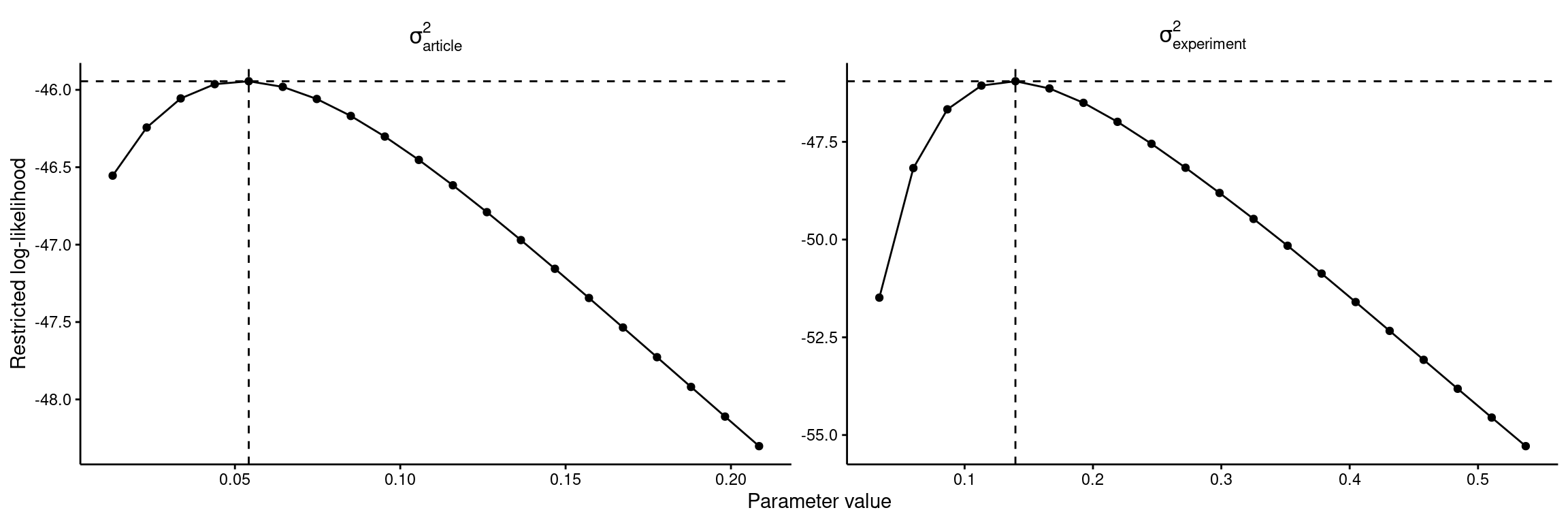
# Get profile likelihoods for sigmas to check that REML has converged
prof_liks <- profile(res_freq_meta, plot = FALSE)

# Combine frequentist profile likelihood results into one data frame
prof_liks_df <- prof_liks %>%
  head(-1) %>% # Remove the `comp` element
  map(~ tibble(sigma2 = .$sigma2, ll = .$ll)) %>%
  bind_rows(.id = "parameter") %>%
  # Create new labels for plotting
  mutate(parameter = factor(
    parameter,
    levels = c(1, 2),
    labels = c("italic(sigma)[article]^2", "italic(sigma)[experiment]^2")
  ))

# Find the best-fitting parameter estimates
prof_liks_max <- prof_liks_df %>%
  group_by(parameter) %>%
  filter(ll == max(ll))

# Create plot
prof_liks_df %>%
  ggplot(aes(x = sigma2, y = ll)) +
  facet_wrap(~parameter, scales = "free", labeller = label_parsed) +
  # Best fitting parameters
  geom_hline(
    aes(yintercept = ll),
    data = prof_liks_max, linetype = "dashed"
  ) +
  geom_vline(
    aes(xintercept = sigma2),
    data = prof_liks_max, linetype = "dashed"
  ) +
  # All tested parameters
  geom_point() +
  geom_line() +
  # Styling
  labs(x = "Parameter value", y = "Restricted log-likelihood") +
  theme_classic() +
  theme(
    axis.line = element_line(colour = "black"),
    axis.text = element_text(family = "Helvetica", color = "black"),
    axis.ticks = element_line(color = "black"),
    strip.background = element_blank(),
    strip.text = element_text(family = "Helvetica", color = "black", size = 12),
    text = element_text(family = "Helvetica", color = "black")
  )

# Save the plot
ggsave(here(figures_dir, "figs2_convergence_freq.pdf"), width = 12, height = 4)

Profiling sigma2 = 1 
Profiling sigma2 = 2 

2.4.2 Trim-and-fill plot

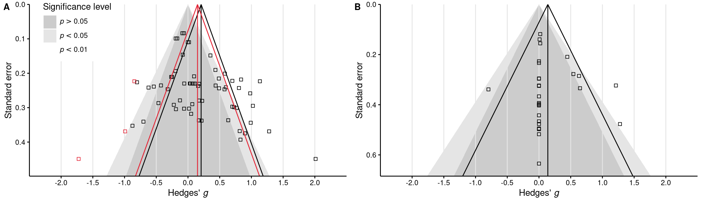
Funnel plot for trim-and-fill model (Supplementary Figure 3)

Code

# Create new funnel plots that take the trim-and-fill results into account
plots_funnel_trim_fill <- map2(
  res_trim_fill, plots_funnel,
  function(res, plot) {
    # Compute new funnel
    funnel_trim_fill <- with(
      list(
        z_crit_05 = stats::qnorm(0.975),
        max_se = max(sqrt(res$vi)) + 0.05
      ),
      {
        data.frame(
          x = c(
            res$b - z_crit_05 * sqrt(max_se^2),
            res$b,
            res$b + z_crit_05 * sqrt(max_se^2)
          ),
          y = c(max_se, 0, max_se)
        )
      }
    )

    # Add new funnel on top of the original funnel plot
    trim_fill_color <- ifelse(sum(res$fill) >= 1, "#e42536", NA)
    plot +
      # Add trim-and-fill funnel
      geom_path(
        data = funnel_trim_fill,
        aes(x = x, y = y),
        color = trim_fill_color
      ) +
      geom_vline(xintercept = res$b, color = trim_fill_color) +
      # Add trim-and-fill studies
      geom_point(
        data = with(res, tibble(gi = yi[fill], sei = sqrt(vi[fill]))),
        color = trim_fill_color, shape = 0
      )
  }
)

# Combine plots and legend
plot_grid(
  plotlist = plots_funnel_trim_fill, nrow = 1, labels = "AUTO",
  label_size = 11, label_fontfamily = "Helvetica"
) +
  draw_plot(legend_funnel, x = -0.39, y = 0.355)

# Save the plot
ggsave(
  here(figures_dir, "figs3_funnel_trim_fill.pdf"),
  width = 12, height = 3.5
)

2.4.3 Meta-analysis of gender differences

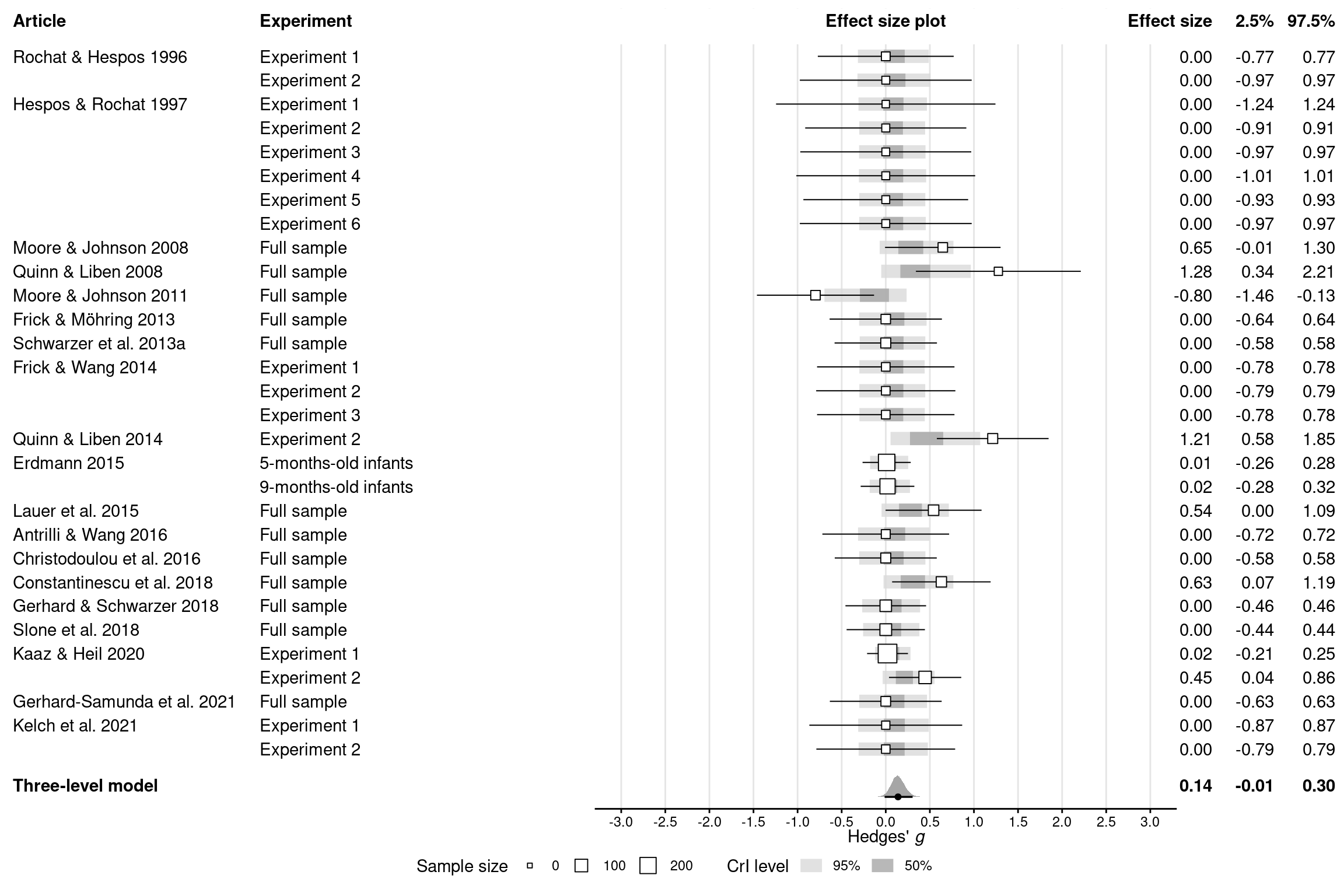
Forest plot (Supplementary Figure 4)

Code

# Get posterior draws for the effect *in each experiment*
epred_draws_gender <- epred_draws(res_gender, dat_gender, ndraws = NULL) %>%
  mutate(experiment_f = factor(experiment))

# Create forest plot
dat_gender %>%
  # Make sure the plot will be ordered alphabetically by experiment IDs
  arrange(experiment) %>%
  mutate(
    experiment_f = fct_rev(fct_expand(factor(experiment), "model")),
    # Show article labels only for the first experiment (row) per article
    article = if_else(article == lag(article, default = ""), "", article),
    # Compute frequentist confidence intervals
    ci_lb = gi - qnorm(0.05 / 2, lower.tail = FALSE) * sqrt(vi),
    ci_ub = gi + qnorm(0.05 / 2, lower.tail = FALSE) * sqrt(vi),
    ci_print = print_mean_ci(gi, ci_lb, ci_ub)
  ) %>%
  # Prepare plotting canvas
  ggplot(aes(x = gi, y = experiment_f)) +
  geom_vline(xintercept = seq(-3, 3, 0.5), color = "grey90") +
  # Add article and group labels as text on the left
  geom_text(aes(x = -9.9, label = article), hjust = 0) +
  geom_text(aes(x = -7.1, label = group), hjust = 0) +
  # Add experiment-specific effect sizes and CIs as text on the right
  geom_text(aes(x = 3.7, label = print_num(gi)), hjust = 1) +
  geom_text(aes(x = 4.4, label = print_num(ci_lb)), hjust = 1) +
  geom_text(aes(x = 5.1, label = print_num(ci_ub)), hjust = 1) +
  # Add Bayesian credible intervals for each experiment
  stat_interval(
    aes(x = .epred),
    data = epred_draws_gender,
    alpha = .8,
    point_interval = "mean_qi",
    .width = c(0.5, 0.95),
  ) +
  scale_color_grey(
    start = 0.85, end = 0.65,
    labels = as_mapper(~ scales::percent(as.numeric(.x)))
  ) +
  # Add experiment-specific effect sizes and CIs as dots with error bars
  geom_linerange(aes(xmin = ci_lb, xmax = ci_ub), size = 0.35) +
  geom_point(aes(size = ni), shape = 22, fill = "white") + # Or (1 / vi)?
  # Add posterior distribution for the meta-analytic effect
  stat_halfeye(
    aes(x = intercept, y = -1),
    draws_gender,
    point_interval = "mean_qi",
    .width = c(0.95)
  ) +
  annotate(
    "text",
    x = c(-9.9, 3.7, 4.4, 5.1),
    y = -0.5,
    label = c(
      "Three-level model",
      print_num(summ_gender$intercept),
      print_num(summ_gender$intercept.lower),
      print_num(summ_gender$intercept.upper)
    ),
    hjust = c(0, 1, 1, 1),
    fontface = "bold"
  ) +
  # Add column headers
  annotate(
    "rect",
    xmin = -Inf,
    xmax = Inf,
    ymin = nrow(dat_gender) + 0.5,
    ymax = Inf,
    fill = "white"
  ) +
  annotate(
    "text",
    x = c(-9.9, -7.1, 0, 3.7, 4.4, 5.1),
    y = nrow(dat_gender) + 1.5,
    label = c(
      "Article",
      "Experiment",
      "Effect size plot",
      "Effect size",
      "2.5%",
      "97.5%"
    ),
    hjust = c(0, 0, 0.5, 1, 1, 1),
    fontface = "bold"
  ) +
  # Styling
  coord_cartesian(
    ylim = c(-1.5, nrow(dat_gender) + 2), expand = FALSE, clip = "off"
  ) +
  scale_x_continuous(breaks = seq(-3, 3, 0.5)) +
  annotate("segment", x = -3.3, xend = 3.3, y = -1.5, yend = -1.5) +
  labs(
    x = expression("Hedges'" ~ italic("g")),
    size = "Sample size",
    color = "CrI level"
  ) +
  theme_minimal() +
  theme(
    legend.position = "bottom",
    axis.text.x = element_text(family = "Helvetica", color = "black"),
    axis.text.y = element_blank(),
    axis.ticks.x = element_line(colour = "black"),
    axis.title.x = element_text(hjust = 0.67, margin = margin(b = -15)),
    axis.title.y = element_blank(),
    panel.grid = element_blank(),
    text = element_text(family = "Helvetica")
  )

# Save the plot
ggsave(here(figures_dir, "figs4_gender.pdf"), width = 12, height = 8)

2.4.4 Accounting for familiarity preferences

Re-fit meta-analysis of mental rotation performance

Code

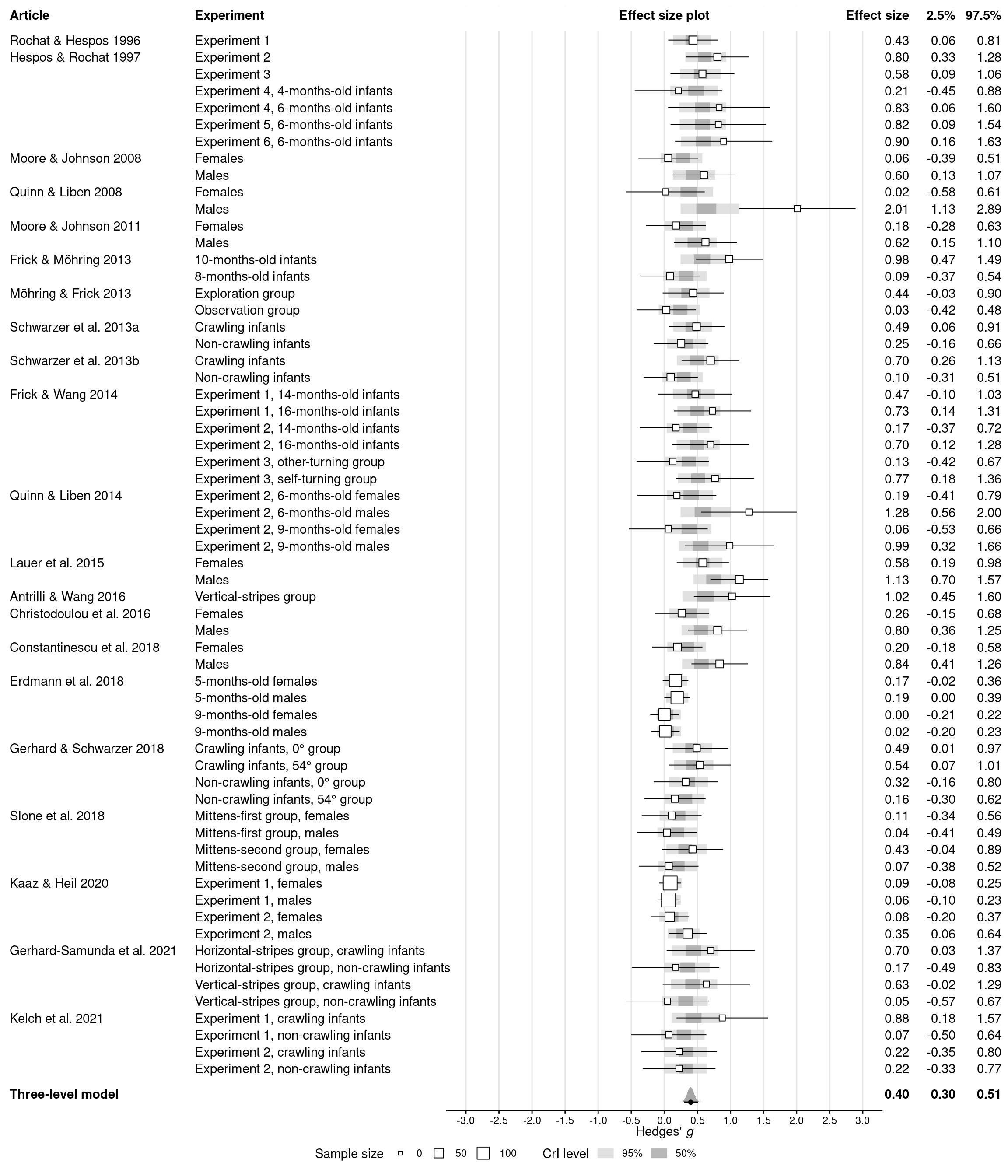
# Re-code familiarity preference to be treated the same as novelty preference
dat_meta_pos <- mutate(dat_meta, gi = abs(gi))

# Specify new priors
prior_meta_pos <- c(
  set_prior("normal(0, 1)", class = "b", lb = 0),
  set_prior("cauchy(0, 0.3)", class = "sd")
)

# Re-fit meta-analysis using the new data and priors
res_meta_pos <- update(
  res_meta,
  newdata = dat_meta_pos,
  prior = prior_meta_pos,
  file = here(models_dir, "res_meta_pos"),
  file_refit = brms_file_refit
)
summary(res_meta_pos)

 Family: gaussian 
  Links: mu = identity; sigma = identity 
Formula: gi | se(sei) ~ 0 + Intercept + (1 | article/experiment) 
   Data: dat_meta_pos (Number of observations: 62) 
  Draws: 4 chains, each with iter = 18000; warmup = 0; thin = 1;
         total post-warmup draws = 72000

Group-Level Effects: 
~article (Number of levels: 21) 
              Estimate Est.Error l-95% CI u-95% CI Rhat Bulk_ESS Tail_ESS
sd(Intercept)     0.15      0.06     0.03     0.26 1.00    15368    15231

~article:experiment (Number of levels: 62) 
              Estimate Est.Error l-95% CI u-95% CI Rhat Bulk_ESS Tail_ESS
sd(Intercept)     0.15      0.07     0.02     0.28 1.00     9660    15105

Population-Level Effects: 
          Estimate Est.Error l-95% CI u-95% CI Rhat Bulk_ESS Tail_ESS
Intercept     0.40      0.05     0.30     0.51 1.00    56395    53113

Family Specific Parameters: 
      Estimate Est.Error l-95% CI u-95% CI Rhat Bulk_ESS Tail_ESS
sigma     0.00      0.00     0.00     0.00   NA       NA       NA

Draws were sampled using sample(hmc). For each parameter, Bulk_ESS
and Tail_ESS are effective sample size measures, and Rhat is the potential
scale reduction factor on split chains (at convergence, Rhat = 1).

Summary of model parameters

Code

# Extract posterior draws for the meta-analytic effects
draws_meta_pos <- spread_draws(
  res_meta_pos, `b_.*`, `sd_.*`,
  regex = TRUE, ndraws = NULL
) %>%
  # Compute variances and ICC from standard deviations
  mutate(
    intercept = b_Intercept,
    sigma_article = sd_article__Intercept,
    sigma_experiment = `sd_article:experiment__Intercept`,
    sigma2_article = sigma_article^2,
    sigma2_experiment = sigma_experiment^2,
    sigma2_total = sigma2_article + sigma2_experiment,
    icc = sigma2_article / sigma2_total,
    .keep = "unused"
  )

# Summarize as means and 95% credible intervals
(summ_meta_pos <- mean_qi(draws_meta_pos))

Forest plot (Supplementary Figure 5)

Code

# Get posterior draws for the effect *in each experiment*
epred_draws_meta_pos <-
  epred_draws(res_meta_pos, dat_meta_pos, ndraws = NULL) %>%
  mutate(experiment_f = factor(experiment))

# Create forest plot
dat_meta_pos %>%
  # Make sure the plot will be ordered alphabetically by experiment IDs
  arrange(experiment) %>%
  mutate(
    experiment_f = fct_rev(fct_expand(factor(experiment), "model")),
    # Show article labels only for the first experiment (row) per article
    article = if_else(article == lag(article, default = ""), "", article),
    # Compute frequentist confidence intervals for each experiment
    ci_lb = gi - qnorm(0.05 / 2, lower.tail = FALSE) * sqrt(vi),
    ci_ub = gi + qnorm(0.05 / 2, lower.tail = FALSE) * sqrt(vi),
    ci_print = print_mean_ci(gi, ci_lb, ci_ub)
  ) %>%
  # Prepare plotting canvas
  ggplot(aes(x = gi, y = experiment_f)) +
  geom_vline(xintercept = seq(-3, 3, 0.5), color = "grey90") +
  # Add article and group labels as text on the left
  geom_text(aes(x = -9.9, label = article), hjust = 0) +
  geom_text(aes(x = -7.1, label = group), hjust = 0) +
  # Add experiment-specific effect sizes and CIs as text on the right
  geom_text(aes(x = 3.7, label = print_num(gi)), hjust = 1) +
  geom_text(aes(x = 4.4, label = print_num(ci_lb)), hjust = 1) +
  geom_text(aes(x = 5.1, label = print_num(ci_ub)), hjust = 1) +
  # Add Bayesian credible intervals for each experiment
  stat_interval(
    aes(x = .epred),
    data = epred_draws_meta_pos,
    alpha = .8,
    point_interval = "mean_qi",
    .width = c(0.5, 0.95),
  ) +
  scale_color_grey(
    start = 0.85, end = 0.65,
    labels = as_mapper(~ scales::percent(as.numeric(.x)))
  ) +
  # Add experiment-specific effect sizes and CIs as dots with error bars
  geom_linerange(aes(xmin = ci_lb, xmax = ci_ub), size = 0.35) +
  geom_point(aes(size = ni), shape = 22, fill = "white") + # Or (1 / vi)?
  # Add posterior distribution for the meta-analytic effect
  stat_halfeye(
    aes(x = intercept, y = -1),
    draws_meta_pos,
    point_interval = "mean_qi",
    .width = c(0.95)
  ) +
  annotate(
    "text",
    x = c(-9.9, 3.7, 4.4, 5.1),
    y = -0.5,
    label = c(
      "Three-level model",
      print_num(summ_meta_pos$intercept),
      print_num(summ_meta_pos$intercept.lower),
      print_num(summ_meta_pos$intercept.upper)
    ),
    hjust = c(0, 1, 1, 1),
    fontface = "bold"
  ) +
  # Add column headers
  annotate(
    "rect",
    xmin = -Inf,
    xmax = Inf,
    ymin = descriptives$n_experiments + 0.5,
    ymax = Inf,
    fill = "white"
  ) +
  annotate(
    "text",
    x = c(-9.9, -7.1, 0, 3.7, 4.4, 5.1),
    y = descriptives$n_experiments + 1.5,
    label = c(
      "Article",
      "Experiment",
      "Effect size plot",
      "Effect size",
      "2.5%",
      "97.5%"
    ),
    hjust = c(0, 0, 0.5, 1, 1, 1),
    fontface = "bold"
  ) +
  # Styling
  coord_cartesian(
    ylim = c(-1.5, descriptives$n_experiments + 2), expand = FALSE, clip = "off"
  ) +
  scale_x_continuous(breaks = seq(-3, 3, 0.5)) +
  annotate("segment", x = -3.3, xend = 3.3, y = -1.5, yend = -1.5) +
  labs(
    x = expression("Hedges'" ~ italic("g")),
    size = "Sample size",
    color = "CrI level"
  ) +
  theme_minimal() +
  theme(
    legend.position = "bottom",
    axis.text.x = element_text(family = "Helvetica", color = "black"),
    axis.text.y = element_blank(),
    axis.ticks.x = element_line(colour = "black"),
    axis.title.x = element_text(hjust = 0.67, margin = margin(b = -15)),
    axis.title.y = element_blank(),
    panel.grid = element_blank(),
    text = element_text(family = "Helvetica")
  )

# Save the plot
ggsave(here(figures_dir, "figs5_meta_pos.pdf"), width = 12, height = 14)

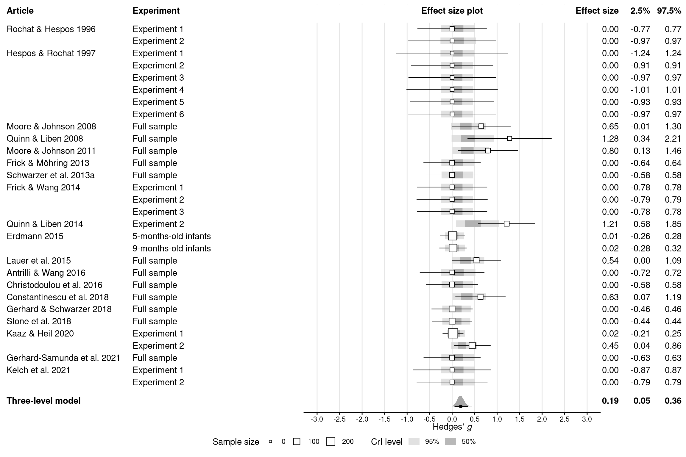
Re-fit meta-analysis of gender differences

Code

# Re-code familiarity preference to be treated the same as novelty preference
dat_gender_pos <- mutate(dat_gender, gi = abs(gi))

# Use the same priors as for the main meta-analysis
prior_gender_pos <- prior_meta_pos

# Re-fit meta-analysis
res_gender_pos <- update(
  res_gender,
  newdata = dat_gender_pos,
  prior = prior_gender_pos,
  file = here(models_dir, "res_gender_pos"),
  file_refit = brms_file_refit
)
summary(res_gender_pos)

 Family: gaussian 
  Links: mu = identity; sigma = identity 
Formula: gi | se(sei) ~ 0 + Intercept + (1 | article/experiment) 
   Data: dat_gender_pos (Number of observations: 30) 
  Draws: 4 chains, each with iter = 18000; warmup = 0; thin = 1;
         total post-warmup draws = 72000

Group-Level Effects: 
~article (Number of levels: 19) 
              Estimate Est.Error l-95% CI u-95% CI Rhat Bulk_ESS Tail_ESS
sd(Intercept)     0.15      0.10     0.01     0.37 1.00    19666    32315

~article:experiment (Number of levels: 30) 
              Estimate Est.Error l-95% CI u-95% CI Rhat Bulk_ESS Tail_ESS
sd(Intercept)     0.11      0.08     0.00     0.29 1.00    25014    31061

Population-Level Effects: 
          Estimate Est.Error l-95% CI u-95% CI Rhat Bulk_ESS Tail_ESS
Intercept     0.19      0.08     0.05     0.36 1.00    41333    29845

Family Specific Parameters: 
      Estimate Est.Error l-95% CI u-95% CI Rhat Bulk_ESS Tail_ESS
sigma     0.00      0.00     0.00     0.00   NA       NA       NA

Draws were sampled using sample(hmc). For each parameter, Bulk_ESS
and Tail_ESS are effective sample size measures, and Rhat is the potential
scale reduction factor on split chains (at convergence, Rhat = 1).

Summary of model paramters

Code

# Extract posterior draws for the meta-analytic effects
draws_gender_pos <- spread_draws(
  res_gender_pos, `b_.*`, `sd_.*`,
  regex = TRUE, ndraws = NULL
) %>%
  # Compute variances and ICC from standard deviations
  mutate(
    intercept = b_Intercept,
    sigma_article = sd_article__Intercept,
    sigma_experiment = `sd_article:experiment__Intercept`,
    sigma2_article = sigma_article^2,
    sigma2_experiment = sigma_experiment^2,
    sigma2_total = sigma2_article + sigma2_experiment,
    icc = sigma2_article / sigma2_total,
    .keep = "unused"
  )

# Summarize as means and 95% credible intervals
(summ_gender_pos <- mean_qi(draws_gender_pos))

Forest plot (Supplementary Figure 6)

Code

# Get posterior draws for the effect *in each experiment*
epred_draws_gender_pos <-
  epred_draws(res_gender_pos, dat_gender_pos, ndraws = NULL) %>%
  mutate(experiment_f = factor(experiment))

# Create forest plot
dat_gender_pos %>%
  # Make sure the plot will be ordered alphabetically by experiment IDs
  arrange(experiment) %>%
  mutate(
    experiment_f = fct_rev(fct_expand(factor(experiment), "model")),
    # Show article labels only for the first experiment (row) per article
    article = if_else(article == lag(article, default = ""), "", article),
    # Compute frequentist confidence intervals
    ci_lb = gi - qnorm(0.05 / 2, lower.tail = FALSE) * sqrt(vi),
    ci_ub = gi + qnorm(0.05 / 2, lower.tail = FALSE) * sqrt(vi),
    ci_print = print_mean_ci(gi, ci_lb, ci_ub)
  ) %>%
  # Prepare plotting canvas
  ggplot(aes(x = gi, y = experiment_f)) +
  geom_vline(xintercept = seq(-3, 3, 0.5), color = "grey90") +
  # Add article and group labels as text on the left
  geom_text(aes(x = -9.9, label = article), hjust = 0) +
  geom_text(aes(x = -7.1, label = group), hjust = 0) +
  # Add experiment-specific effect sizes and CIs as text on the right
  geom_text(aes(x = 3.7, label = print_num(gi)), hjust = 1) +
  geom_text(aes(x = 4.4, label = print_num(ci_lb)), hjust = 1) +
  geom_text(aes(x = 5.1, label = print_num(ci_ub)), hjust = 1) +
  # Add Bayesian credible intervals for each experiment
  stat_interval(
    aes(x = .epred),
    data = epred_draws_gender_pos,
    alpha = .8,
    point_interval = "mean_qi",
    .width = c(0.5, 0.95),
  ) +
  scale_color_grey(
    start = 0.85, end = 0.65,
    labels = as_mapper(~ scales::percent(as.numeric(.x)))
  ) +
  # Add experiment-specific effect sizes and CIs as dots with error bars
  geom_linerange(aes(xmin = ci_lb, xmax = ci_ub), size = 0.35) +
  geom_point(aes(size = ni), shape = 22, fill = "white") + # Or (1 / vi)?
  # Add posterior distribution for the meta-analytic effect
  stat_halfeye(
    aes(x = intercept, y = -1),
    draws_gender_pos,
    point_interval = "mean_qi",
    .width = c(0.95)
  ) +
  annotate(
    "text",
    x = c(-9.9, 3.7, 4.4, 5.1),
    y = -0.5,
    label = c(
      "Three-level model",
      print_num(summ_gender_pos$intercept),
      print_num(summ_gender_pos$intercept.lower),
      print_num(summ_gender_pos$intercept.upper)
    ),
    hjust = c(0, 1, 1, 1),
    fontface = "bold"
  ) +
  # Add column headers
  annotate(
    "rect",
    xmin = -Inf,
    xmax = Inf,
    ymin = nrow(dat_gender_pos) + 0.5,
    ymax = Inf,
    fill = "white"
  ) +
  annotate(
    "text",
    x = c(-9.9, -7.1, 0, 3.7, 4.4, 5.1),
    y = nrow(dat_gender_pos) + 1.5,
    label = c(
      "Article",
      "Experiment",
      "Effect size plot",
      "Effect size",
      "2.5%",
      "97.5%"
    ),
    hjust = c(0, 0, 0.5, 1, 1, 1),
    fontface = "bold"
  ) +
  # Styling
  coord_cartesian(
    ylim = c(-1.5, nrow(dat_gender_pos) + 2), expand = FALSE, clip = "off"
  ) +
  scale_x_continuous(breaks = seq(-3, 3, 0.5)) +
  annotate("segment", x = -3.3, xend = 3.3, y = -1.5, yend = -1.5) +
  labs(
    x = expression("Hedges'" ~ italic("g")),
    size = "Sample size",
    color = "CrI level"
  ) +
  theme_minimal() +
  theme(
    legend.position = "bottom",
    axis.text.x = element_text(family = "Helvetica", color = "black"),
    axis.text.y = element_blank(),
    axis.ticks.x = element_line(colour = "black"),
    axis.title.x = element_text(hjust = 0.67, margin = margin(b = -15)),
    axis.title.y = element_blank(),
    panel.grid = element_blank(),
    text = element_text(family = "Helvetica")
  )

# Save the plot
ggsave(here(figures_dir, "figs6_gender_pos.pdf"), width = 12, height = 8)

2.5 References

Cumming, Geoff. 2012. Understanding the New Statistics: Effect Sizes, Confidence Intervals, and Meta-Analysis. Multivariate Applications Series. New York: Routledge.

Goulet-Pelletier, Jean-Christophe, and Denis Cousineau. 2018. “A Review of Effect Sizes and Their Confidence Intervals, Part I: The Cohen’s d Family.” The Quantitative Methods for Psychology 14 (4): 242–65. https://doi.org/10.20982/tqmp.14.4.p242.

Hedges, Larry V., and Ingram Olkin. 1985. Statistical Methods for Meta-Analysis. San Diego: Academic Press.

Lakens, Daniel. 2013. “Calculating and Reporting Effect Sizes to Facilitate Cumulative Science: A Practical Primer for t-Tests and ANOVAs.” Frontiers in Psychology 4. https://doi.org/10.3389/fpsyg.2013.00863.

Rosenthal, Robert. 1991. Meta-Analytic Procedures for Social Research. Meta-Analytic Procedures for Social Research, Rev. Ed. Thousand Oaks, CA, US: SAGE Publications.