# Load packageslibrary(papaja)library(here)library(scales)library(tidyverse)library(furrr)library(metafor)library(brms)library(tidybayes)library(cowplot)# Load custom helper functionssource(here("misc", "helper_functions.R"))# Re-run steps that take a long time?run <-list(bayesian_models =FALSE,jackknife_analysis =FALSE,sensitivity_analysis =FALSE)# Options for MCMC sampling when fitting Bayesian multilevel modelsoptions(brms.backend ="cmdstanr") # Can choose "rstan" insteadoptions(mc.cores = parallel::detectCores()) # Use all available coresn_iter <-20000# Posterior samples per chain, including `n_warmup`n_warmup <-2000# Warmup samples per chainn_chains <-4# Number of (parallel) chainsseed <-1234# Random seed to make the results reproducible# Directory pathsdata_dir <-here("data")results_dir <-here("results")models_dir <-here(results_dir, "models")figures_dir <-here(results_dir, "figures")tables_dir <-here(results_dir, "tables")
1.2 Introduction / Methods
1.2.1 Protocol
PRISMA flowchart (Figure 1)
PRISMA flowchart
1.2.2 Selection process
Percent agreement for binary decision (include vs. exclude)
Code
# Read the raw data from the screening processraw_screen <-read_tsv(here(data_dir, "02_screen.tsv"), na ="NA")# Percent agreement for binary decision (include vs. exclude)with(raw_screen, mean(bin_1 == bin_2))
Call: cohen.kappa1(x = x, w = w, n.obs = n.obs, alpha = alpha, levels = levels)

Cohen Kappa and Weighted Kappa correlation coefficients and confidence boundaries
                 lower estimate upper
unweighted kappa  0.69     0.72  0.75
weighted kappa    0.40     0.72  1.00

 Number of subjects = 2037
1.2.3 Effect measures
Conversion of effect sizes for mental rotation performance
Code
# Read raw data for the meta-analysis of mental rotation performanceraw_meta <-read_tsv(here(data_dir, "03_meta.tsv"), na ="NA")# Add columns to the table of experimentsdat_all <- raw_meta %>%mutate(# Add unique experiment identifierexperiment =str_c(year, article, group, sep =", "),# Add difference between condition meansmean_diff =case_when(!is.na(mean_diff) ~ mean_diff,TRUE~ mean_novel - mean_familiar ),# Add d_z from paired-samples t-test of condition means (Rosenthal, 1991)d_z_t = t /sqrt(sample_size),# Add d_z from ANOVA F statistic via conversion to a t statisticd_z_f =sqrt(f) /sqrt(sample_size) * sign_f,# Add d_z from mean and standard deviation of the differenced_z_diff = mean_diff / sd_diff,# Add d_av from mean difference and standard deviations# See http://dx.doi.org/10.20982/tqmp.14.4.p242sd_av =sqrt((sd_novel^2+ sd_familiar^2) /2),d_av = mean_diff / sd_av,# Add d from one-sample t-test of novelty preference scoresd_nov_pref = (nov_pref -0.5) / sd_nov_pref,# Choose one type of outcome variable for each experimentdi =case_when(# 1. If d was reported directed!is.na(d) ~ d,# 2. If a paired-samples t-test was reported!is.na(d_z_t) ~ d_z_t,# 3. If an ANOVA was reported!is.na(d_z_f) ~ d_z_f,# 4. If the difference between means and its SD were reported!is.na(d_z_diff) ~ d_z_diff,# 5. If the individual condition means and their SDs were reported!is.na(d_av) ~ d_av,# 6. If a novelty preference score and its SD were reported!is.na(d_nov_pref) ~ d_nov_pref ),# Keep track which type of outcome measure was chosen for each articledi_type =case_when(!is.na(d) ~"d",!is.na(d_z_t) ~"d_z_t",!is.na(d_z_f) ~"d_z_f",!is.na(d_z_diff) ~"d_z_diff",!is.na(d_av) ~"d_av",!is.na(d_nov_pref) ~"d_nov_pref",TRUE~"none" ) %>%factor(levels =c("d", "d_z_t", "d_z_f", "d_z_diff", "d_av", "d_nov_pref", "none" )),# Apply small sample correction using Hedges' exact method# See http://dx.doi.org/10.20982/tqmp.14.4.p242dfi =2* (sample_size -1),ji =exp(lgamma(dfi /2) -log(sqrt(dfi /2)) -lgamma((dfi -1) /2)),gi = di * ji,# Recode gender as a categorical (factor) variable for meta-regressiongender =case_when( female_percent ==1.0~"Female", female_percent ==0.0~"Male",TRUE~"Mixed" ) %>%factor(levels =c("Mixed", "Female", "Male")),# Recode mean sample age in years (mean-centered) for meta-regressionage = age_mean /365.25,age_c = age -mean(age, na.rm =TRUE),# Recode task type as a categorical (factor) variable for meta-regressiontask =factor(task, levels =c("Habituation", "VoE")),# Combine gender and task into one column for plottinggender_task =factor(str_c(gender, task, sep =", "),levels =c("Female, Habituation","Male, Habituation","Mixed, Habituation","Mixed, VoE" ) ) ) %>%# Order rows by experiment IDarrange(experiment)# Compute standard errors of the effect sizes based on assumed correlation# See Hedges' formula on p. 253 in http://dx.doi.org/10.20982/tqmp.14.4.p242# You'll find a sensitivity analysis for `r_assumed` in the `supplement.Rmd`r_assumed <-0.5dat_meta_all <- dat_all %>%mutate(ni = sample_size,vi = (dfi / (dfi -2)) * ((2* (1- r_assumed)) / ni) * (1+ gi^2* (ni / (2* (1- r_assumed)))) - (gi^2/ ji^2),sei =sqrt(vi) ) %>%filter(!is.na(gi))# Extract either split or mixed experiments onlydat_split <-filter(dat_meta_all, gender_split %in%c("split", "split_only"))dat_mixed <-filter(dat_meta_all, gender_split %in%c("mixed", "mixed_only"))# Combine both strategies but preferring mixed experimentsdat_both_mixed <-filter( dat_meta_all, gender_split %in%c("mixed", "mixed_only", "split_only"))# Combine both strategies but preferring split experimentsdat_both_split <-filter( dat_meta_all, gender_split %in%c("split", "mixed_only", "split_only"))# We go ahead with the last solution (i.e., prefer split experiments) as to use# the maximum amount of information while not biasing the gender resultsdat_meta <- dat_both_split
Conversion of effect sizes for gender differences
Code
# Read raw data for the meta-analysis of gender differencesraw_gender <-read_tsv(here(data_dir, "04_gender.tsv"), na ="NA")# Compute relevant effect sizes for the meta-analysis of gender differencesdat_gender <- raw_gender %>%# Remove effect sizes from experiments with redundant samplesfilter(!redundant) %>%# Add columnsmutate(# Add unique experiment identifierexperiment =str_c(year, article, group, sep =", "),# Re-code non-significant F statistics as an effect size of d = 0f =as.numeric(f),f_assumed =ifelse(is.nan(f), 0, f),# Add d from two-samples t-test (Lakens, 2013)d_t = t *sqrt(1/ female_n +1/ male_n),# Add d from ANOVA F statistic via conversion to a t statisticd_f =sqrt(f_assumed) * sign_f *sqrt(1/ female_n +1/ male_n),# Add d from mean difference and pooled standard deviationmean_diff = mean_diff_males_mean - mean_diff_females_mean,sd_diff_pooled_numerator = (male_n -1) * (mean_diff_males_sd^2) + (female_n -1) * (mean_diff_females_sd^2),df = male_n + female_n -2,sd_diff_pooled =sqrt(sd_diff_pooled_numerator / df),d_diff = mean_diff / sd_diff_pooled,# Add d from one-sample t-test of novelty preference scoresmean_nov_pref = novelty_pref_males_mean - novelty_pref_females_mean,sd_nov_pref_pooled_numerator = (male_n -1) * (novelty_pref_males_sd^2) + (female_n) * (novelty_pref_females_sd^2),sd_nov_pref_pooled =sqrt(sd_nov_pref_pooled_numerator / df),d_nov_pref = mean_nov_pref / sd_nov_pref_pooled,# Choose one type of outcome variable for each experimentdi =case_when(# 1. If d was reported directed!is.na(d) ~ d,# 2. If a t-test was reported!is.na(d_t) ~ d_t,# 3. If an ANOVA was reported!is.na(d_f) ~ d_f,# 4. If the difference between means and their SDs were reported!is.na(d_diff) ~ d_diff,# 5. If novelty preference scores and their SDs were reported!is.na(d_nov_pref) ~ d_nov_pref ),# Keep track which type of outcome measure was chosen for each articledi_type =case_when(!is.na(d) ~"d",!is.na(d_t) ~"d_t",!is.na(d_f) ~"d_f",!is.na(d_diff) ~"d_diff",!is.na(d_nov_pref) ~"d_nov_pref" ) %>%factor(levels =c("d", "d_t", "d_f", "d_diff", "d_nov_pref")),# Apply small sample correction using Hedges' exact method# See http://dx.doi.org/10.20982/tqmp.14.4.p242j =exp(lgamma(df /2) -log(sqrt(df /2)) -lgamma((df -1) /2)),gi = di * j,# Compute standard error of Cohen's d, using harmonic mean of sample sizesni = female_n + male_n,nhi =2/ (1/ female_n +1/ male_n),vi = (df / (df -2)) * (2/ nhi) * (1+ gi^2* (nhi /2)) - (gi^2/ (j^2)),sei =sqrt(vi) ) %>%# Remove experiments that didn't provide any effect sizefilter(!is.na(gi))
Justification for excluding the Pedrett et al. (2020) paper
Code
# Justify exclusion of @pedrett2020 based on outlier mean agedescs_pedrett2020 <-list(age_years =2.56)within(descs_pedrett2020, { age_months <- age_years *12 next_largest_age_months <-max(dat_meta$age_mean) /30.417 age <- age_years *365.25 z <- (age -mean(dat_meta$age_mean)) /sd(dat_meta$age_mean)})
 Family: gaussian
  Links: mu = identity; sigma = identity
Formula: gi | se(sei) ~ 0 + Intercept + (1 | article/experiment)
   Data: dat_meta (Number of observations: 62)
  Draws: 4 chains, each with iter = 18000; warmup = 0; thin = 1;
         total post-warmup draws = 72000

Group-Level Effects:
~article (Number of levels: 21)
              Estimate Est.Error l-95% CI u-95% CI Rhat Bulk_ESS Tail_ESS
sd(Intercept)     2.39    102.73     0.01     7.87 1.00   126795    38369

~article:experiment (Number of levels: 62)
              Estimate Est.Error l-95% CI u-95% CI Rhat Bulk_ESS Tail_ESS
sd(Intercept)     2.21     49.83     0.01     7.89 1.00   101352    38715

Population-Level Effects:
          Estimate Est.Error l-95% CI u-95% CI Rhat Bulk_ESS Tail_ESS
Intercept     0.00      1.00    -1.96     1.95 1.00   143113    53440

Family Specific Parameters:
      Estimate Est.Error l-95% CI u-95% CI Rhat Bulk_ESS Tail_ESS
sigma     0.00      0.00     0.00     0.00   NA       NA       NA

Draws were sampled using sample(hmc). For each parameter, Bulk_ESS
and Tail_ESS are effective sample size measures, and Rhat is the potential
scale reduction factor on split chains (at convergence, Rhat = 1).
 Family: gaussian
  Links: mu = identity; sigma = identity
Formula: gi | se(sei) ~ 0 + Intercept + (1 | article/experiment)
   Data: dat_meta (Number of observations: 62)
  Draws: 4 chains, each with iter = 18000; warmup = 0; thin = 1;
         total post-warmup draws = 72000

Group-Level Effects:
~article (Number of levels: 21)
              Estimate Est.Error l-95% CI u-95% CI Rhat Bulk_ESS Tail_ESS
sd(Intercept)     0.20      0.10     0.02     0.40 1.00     8462    14409

~article:experiment (Number of levels: 62)
              Estimate Est.Error l-95% CI u-95% CI Rhat Bulk_ESS Tail_ESS
sd(Intercept)     0.38      0.07     0.26     0.51 1.00    15520    32722

Population-Level Effects:
          Estimate Est.Error l-95% CI u-95% CI Rhat Bulk_ESS Tail_ESS
Intercept     0.21      0.08     0.06     0.37 1.00    34164    34417

Family Specific Parameters:
      Estimate Est.Error l-95% CI u-95% CI Rhat Bulk_ESS Tail_ESS
sigma     0.00      0.00     0.00     0.00   NA       NA       NA

Draws were sampled using sample(hmc). For each parameter, Bulk_ESS
and Tail_ESS are effective sample size measures, and Rhat is the potential
scale reduction factor on split chains (at convergence, Rhat = 1).
“Test” posterior probability mass above/below zero
Code
# Get posterior probability mass > 0 for the meta-analytic effecthypothesis(res_meta, "Intercept > 0")$hypothesis
Summary of model paramters incl. 95% credible interval (CrI)
Code
# Extract posterior draws for the meta-analytic effectsdraws_meta <-spread_draws( res_meta, `b_.*`, `sd_.*`,regex =TRUE, ndraws =NULL) %>%# Compute variances and ICC from standard deviationsmutate(intercept = b_Intercept,sigma_article = sd_article__Intercept,sigma_experiment =`sd_article:experiment__Intercept`,sigma2_article = sigma_article^2,sigma2_experiment = sigma_experiment^2,sigma2_total = sigma2_article + sigma2_experiment,icc = sigma2_article / sigma2_total,.keep ="unused" )# Summarize as means and 95% credible intervals(summ_meta <-mean_qi(draws_meta))
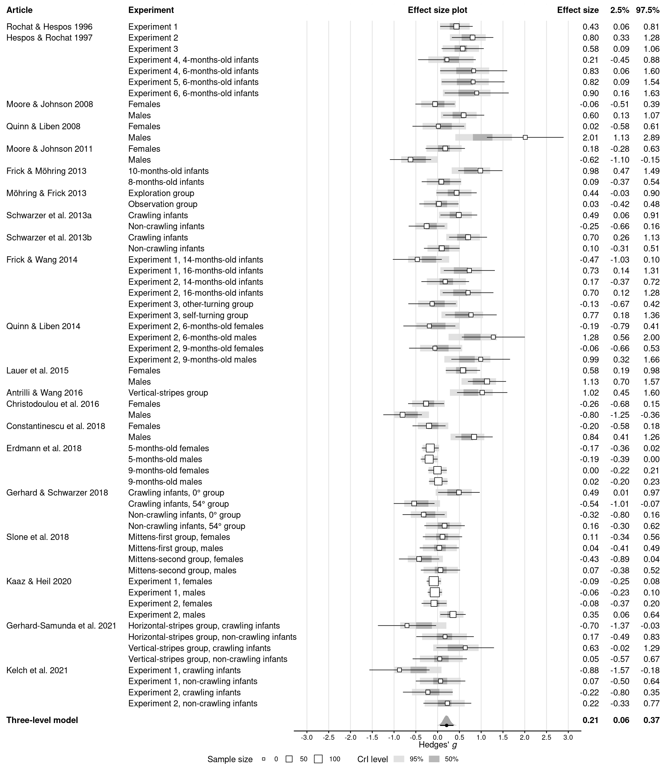
Forest plot (Figure 2)
Code
# Get posterior draws for the effect *in each experiment*epred_draws_meta <-epred_draws(res_meta, dat_meta, ndraws =NULL) %>%mutate(experiment_f =factor(experiment))# Create forest plotdir.create(figures_dir, showWarnings =FALSE)dat_meta %>%# Make sure the plot will be ordered alphabetically by experiment IDsarrange(experiment) %>%mutate(experiment_f =fct_rev(fct_expand(factor(experiment), "model")),# Show article labels only for the first experiment (row) per articlearticle =if_else(article ==lag(article, default =""), "", article),# Compute frequentist confidence intervals for each experimentci_lb = gi -qnorm(0.05/2, lower.tail =FALSE) *sqrt(vi),ci_ub = gi +qnorm(0.05/2, lower.tail =FALSE) *sqrt(vi),ci_print =print_mean_ci(gi, ci_lb, ci_ub) ) %>%# Prepare plotting canvasggplot(aes(x = gi, y = experiment_f)) +geom_vline(xintercept =seq(-3, 3, 0.5), color ="grey90") +# Add article and group labels as text on the leftgeom_text(aes(x =-9.9, label = article), hjust =0) +geom_text(aes(x =-7.1, label = group), hjust =0) +# Add experiment-specific effect sizes and CIs as text on the rightgeom_text(aes(x =3.7, label =print_num(gi)), hjust =1) +geom_text(aes(x =4.4, label =print_num(ci_lb)), hjust =1) +geom_text(aes(x =5.1, label =print_num(ci_ub)), hjust =1) +# Add Bayesian credible intervals for each experimentstat_interval(aes(x = .epred),data = epred_draws_meta,alpha = .8,point_interval ="mean_qi",.width =c(0.5, 0.95), ) +scale_color_grey(start =0.85, end =0.65,labels =as_mapper(~ scales::percent(as.numeric(.x))) ) +# Add experiment-specific effect sizes and CIs as dots with error barsgeom_linerange(aes(xmin = ci_lb, xmax = ci_ub), size =0.35) +geom_point(aes(size = ni), shape =22, fill ="white") +# Or (1 / vi)?# Add posterior distribution for the meta-analytic effectstat_halfeye(aes(x = intercept, y =-1), draws_meta,point_interval ="mean_qi",.width =c(0.95) ) +annotate("text",x =c(-9.9, 3.7, 4.4, 5.1),y =-0.5,label =c("Three-level model",print_num(summ_meta$intercept),print_num(summ_meta$intercept.lower),print_num(summ_meta$intercept.upper) ),hjust =c(0, 1, 1, 1),fontface ="bold" ) +# Add column headersannotate("rect",xmin =-Inf,xmax =Inf,ymin = descriptives$n_experiments +0.5,ymax =Inf,fill ="white" ) +annotate("text",x =c(-9.9, -7.1, 0, 3.7, 4.4, 5.1),y = descriptives$n_experiments +1.5,label =c("Article","Experiment","Effect size plot","Effect size","2.5%","97.5%" ),hjust =c(0, 0, 0.5, 1, 1, 1),fontface ="bold" ) +# Stylingcoord_cartesian(ylim =c(-1.5, descriptives$n_experiments +2), expand =FALSE,clip ="off" ) +scale_x_continuous(breaks =seq(-3, 3, 0.5)) +annotate("segment", x =-3.3, xend =3.3, y =-1.5, yend =-1.5) +labs(x =expression("Hedges'"~italic("g")),size ="Sample size",color ="CrI level" ) +theme_minimal() +theme(legend.position ="bottom",axis.text.x =element_text(family ="Helvetica", color ="black"),axis.text.y =element_blank(),axis.ticks.x =element_line(colour ="black"),axis.title.x =element_text(hjust =0.67, margin =margin(b =-15)),axis.title.y =element_blank(),panel.grid =element_blank(),text =element_text(family ="Helvetica") )# Save the plotdir.create(figures_dir, showWarnings =FALSE)ggsave(here(figures_dir, "fig2_meta.pdf"), width =12, height =14)
1.3.2 Effects of gender, age, and task type
Prior predictive check
Code
# Set numerical contrasts for factor variablescontrasts(dat_meta$gender) <- MASS::contr.sdif(3)contrasts(dat_meta$task) <- MASS::contr.sdif(2)# Specify priorsprior_reg <-c(set_prior("normal(0, 1)", class ="b", coef ="Intercept"),set_prior("normal(0, 0.5)", class ="b"),set_prior("cauchy(0, 0.3)", class ="sd"))# Run prior predictive simulationres_prior_reg <-brm( gi |se(sei) ~0+ Intercept + gender * age_c + task + (1| article / experiment),data = dat_meta,prior = prior_reg,sample_prior ="only",save_pars =save_pars(all =TRUE),chains = n_chains,iter = n_iter,warmup = n_warmup,cores = n_chains,control =list(adapt_delta =0.99),seed = seed,file =here(models_dir, "res_prior_reg"),file_refit = brms_file_refit)summary(res_prior_reg)
 Family: gaussian
  Links: mu = identity; sigma = identity
Formula: gi | se(sei) ~ 0 + Intercept + gender * age_c + task + (1 | article/experiment)
   Data: dat_meta (Number of observations: 62)
  Draws: 4 chains, each with iter = 18000; warmup = 0; thin = 1;
         total post-warmup draws = 72000

Group-Level Effects:
~article (Number of levels: 21)
              Estimate Est.Error l-95% CI u-95% CI Rhat Bulk_ESS Tail_ESS
sd(Intercept)     2.13     81.77     0.01     7.56 1.00   123575    42711

~article:experiment (Number of levels: 62)
              Estimate Est.Error l-95% CI u-95% CI Rhat Bulk_ESS Tail_ESS
sd(Intercept)     3.96    307.71     0.01     8.36 1.00   122218    40847

Population-Level Effects:
                Estimate Est.Error l-95% CI u-95% CI Rhat Bulk_ESS Tail_ESS
Intercept          -0.00      1.00    -1.96     1.96 1.00   144991    51676
gender2M1          -0.00      0.50    -0.98     0.98 1.00   157626    50676
gender3M2          -0.00      0.50    -0.98     0.98 1.00   140280    52362
age_c              -0.00      0.51    -1.00     1.00 1.00   146045    50860
task2M1            -0.00      0.50    -0.98     0.98 1.00   147301    51698
gender2M1:age_c    -0.00      0.50    -0.98     0.98 1.00   148525    53545
gender3M2:age_c    -0.00      0.50    -0.99     0.98 1.00   141081    50688

Family Specific Parameters:
      Estimate Est.Error l-95% CI u-95% CI Rhat Bulk_ESS Tail_ESS
sigma     0.00      0.00     0.00     0.00   NA       NA       NA

Draws were sampled using sample(hmc). For each parameter, Bulk_ESS
and Tail_ESS are effective sample size measures, and Rhat is the potential
scale reduction factor on split chains (at convergence, Rhat = 1).
 Family: gaussian
  Links: mu = identity; sigma = identity
Formula: gi | se(sei) ~ 0 + Intercept + gender * age_c + task + (1 | article/experiment)
   Data: dat_meta (Number of observations: 62)
  Draws: 4 chains, each with iter = 18000; warmup = 0; thin = 1;
         total post-warmup draws = 72000

Group-Level Effects:
~article (Number of levels: 21)
              Estimate Est.Error l-95% CI u-95% CI Rhat Bulk_ESS Tail_ESS
sd(Intercept)     0.17      0.10     0.01     0.38 1.00     9631    20073

~article:experiment (Number of levels: 62)
              Estimate Est.Error l-95% CI u-95% CI Rhat Bulk_ESS Tail_ESS
sd(Intercept)     0.35      0.06     0.23     0.47 1.00    19254    32563

Population-Level Effects:
                Estimate Est.Error l-95% CI u-95% CI Rhat Bulk_ESS Tail_ESS
Intercept           0.33      0.10     0.14     0.53 1.00    30155    34600
gender2M1          -0.02      0.19    -0.38     0.36 1.00    32744    39842
gender3M2           0.32      0.15     0.02     0.62 1.00    32409    42739
age_c               0.33      0.29    -0.24     0.90 1.00    43588    49680
task2M1             0.38      0.18     0.01     0.73 1.00    34466    37847
gender2M1:age_c     0.15      0.41    -0.66     0.96 1.00    48925    49252
gender3M2:age_c     0.17      0.42    -0.66     0.99 1.00    66057    52582

Family Specific Parameters:
      Estimate Est.Error l-95% CI u-95% CI Rhat Bulk_ESS Tail_ESS
sigma     0.00      0.00     0.00     0.00   NA       NA       NA

Draws were sampled using sample(hmc). For each parameter, Bulk_ESS
and Tail_ESS are effective sample size measures, and Rhat is the potential
scale reduction factor on split chains (at convergence, Rhat = 1).
“Test” posterior probability mass above/below zero
Code
# Get posterior probability mass > 0 for all regression weightsbind_rows(hypothesis(res_reg, "Intercept > 0")$hypothesis,hypothesis(res_reg, "gender2M1 < 0")$hypothesis,hypothesis(res_reg, "gender3M2 > 0")$hypothesis,hypothesis(res_reg, "age_c > 0")$hypothesis,hypothesis(res_reg, "task2M1 > 0")$hypothesis,hypothesis(res_reg, "gender2M1:age_c > 0")$hypothesis,hypothesis(res_reg, "gender3M2:age_c > 0")$hypothesis)
Summary of model paramters incl. 95% CrI
Code
# Extract posterior draws for the meta-analytic effectsdraws_reg <-spread_draws( res_reg, `b_.*`, `sd_.*`,regex =TRUE, ndraws =NULL) %>%# Compute variances and ICC from standard deviationsmutate(intercept = b_Intercept,female_mixed = b_gender2M1,male_female = b_gender3M2,age = b_age_c,voe_habituation = b_task2M1,female_mixed_age =`b_gender2M1:age_c`,male_female_age =`b_gender3M2:age_c`,sigma_article = sd_article__Intercept,sigma_experiment =`sd_article:experiment__Intercept`,sigma2_article = sd_article__Intercept^2,sigma2_experiment =`sd_article:experiment__Intercept`^2,sigma2_total = sigma2_article + sigma2_experiment,icc = sigma2_article / sigma2_total, )# Summarize as means and 95% credible intervals(summ_reg <-mean_qi(draws_reg))
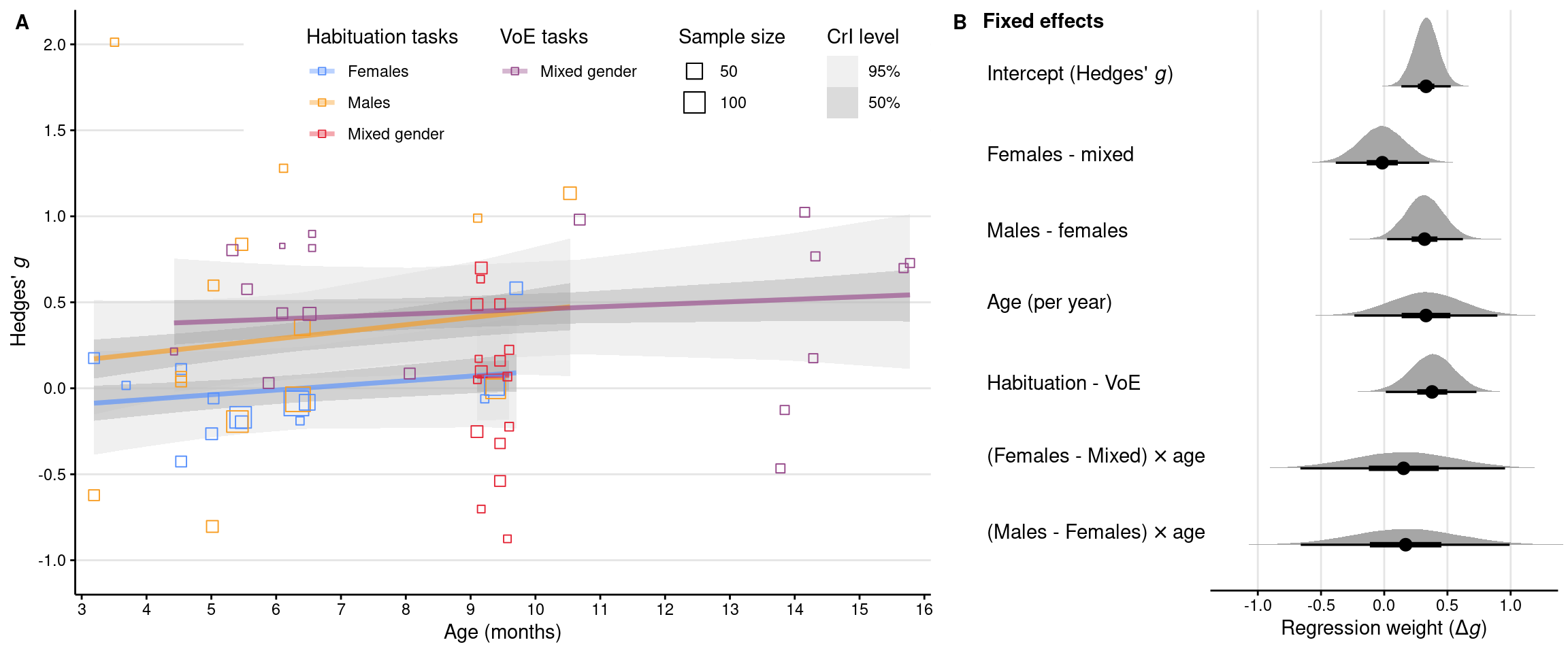
Meta-regression plot (Figure 3)
Code
# Get draws from the posterior distribution *for each experiment*epred_draws_reg <-epred_draws( res_reg, dat_meta,ndraws =NULL,re_formula =NA)# Use colors as proposed in https://arxiv.org/abs/2107.02270# The four colors code for a combination of tasks (Habituation, VoE) and gender# (female, male, mixed)plot_reg_colors <-list(habituation =c("Female, Habituation"="#5790fc","Male, Habituation"="#f89c20","Mixed, Habituation"="#e42536" ),voe =c("Mixed, VoE"="#964a8b"))# Create regression plotplot_reg <- dat_meta %>%ggplot(aes(x = age *12, y = gi)) +geom_hline(yintercept =seq(-1, 2, 0.5), color ="grey90") +annotate("rect",xmin =5.5, xmax =Inf, ymin =1.25, ymax =Inf,color =NA, fill ="white" ) +# Regression lines and CrIs for Habituation tasksstat_lineribbon(aes(y = .epred, color = gender_task),data = epred_draws_reg,alpha = .4,point_interval ="mean_qi",.width =c(0.5, 0.95) ) +# Individual study effect sizes for Habituation tasksgeom_point(aes(color = gender_task, size = ni), shape =0) +scale_color_manual(values = plot_reg_colors$habituation,breaks =names(plot_reg_colors$habituation),labels =c("Females", "Males", "Mixed gender"),na.value =NA ) +guides(color =guide_legend(title ="Habituation tasks",override.aes =list(fill =NA),order =1 )) +# Regression lines and CrIs for VoE tasks ggnewscale::new_scale_color() +stat_lineribbon(aes(y = .epred, color = gender_task),data = epred_draws_reg,fill =NA,alpha = .4,point_interval ="mean_qi",.width =c(0.5, 0.95) ) +# Individual study effect sizes for VoE tasksgeom_point(aes(color = gender_task, size = ni), shape =0) +scale_color_manual(values = plot_reg_colors$voe,breaks =names(plot_reg_colors$voe),labels =c("Mixed gender"),na.value =NA ) +guides(color =guide_legend(title ="VoE tasks", order =2)) +# Stylingcoord_cartesian(expand =FALSE) +scale_x_continuous(limits =c(2.9, 16.1), breaks =seq(3, 16, 1)) +scale_y_continuous(limits =c(-1.2, 2.2), breaks =seq(-1, 2, 0.5)) +scale_fill_grey(start =0.85, end =0.65,labels =as_mapper(~ scales::percent(as.numeric(.x))) ) +labs(x ="Age (months)",y =expression("Hedges'"~italic("g")),fill ="CrI level",size ="Sample size" ) +theme_classic() +theme(axis.text =element_text(family ="Helvetica", color ="black"),axis.ticks =element_line(color ="black"),legend.direction ="vertical",legend.key =element_blank(),legend.position ="none",panel.grid =element_blank(),text =element_text(family ="Helvetica", color ="black") )# Extract the legend so that we can put it inside the plot later onplot_reg_legend <-get_legend(plot_reg +theme(legend.position ="top"))# Define new labels for the regression coefficientscoef_colnames <-c(b_Intercept =expression("Intercept (Hedges'"~italic(g) *")"),b_gender2M1 =expression("Females - mixed"),b_gender3M2 =expression("Males - females"),b_age_c =expression("Age (per year)"),b_task2M1 =expression("Habituation - VoE"),`b_gender2M1:age_c`=expression("(Females - Mixed)"%*%"age"),`b_gender3M2:age_c`=expression("(Males - Females)"%*%"age"))# Plot posterior distributions of the regression coefficientsepred_draws_reg_coef <-tidy_draws(res_reg)plot_coef <- epred_draws_reg_coef %>%# Convert to long formatselect(all_of(names(coef_colnames))) %>%gather() %>%mutate(coef =factor(key, levels =names(coef_colnames))) %>%# Plot coefficients as "half eyes" (mean + CrIs + distribution)ggplot(aes(x = value, y =fct_rev(coef))) +geom_vline(xintercept =seq(-1, 1, 0.5), color ="grey90") +stat_halfeye(point_interval ="mean_qi", .width =c(0.5, 0.95)) +# Stylingcoord_cartesian(xlim =c(-1.25, 1.25), clip ="off") +scale_x_continuous(breaks =seq(-1, 1, 0.5)) +scale_y_discrete(labels = coef_colnames) +labs(x =expression("Regression weight ("* Delta *italic("g") *")")) +annotate("text",label ="Fixed effects", x =-3.175, y =7.86, hjust =0,family ="Helvetica", fontface ="bold", color ="black" ) +theme_minimal() +theme(axis.line.x =element_line(colour ="black"),axis.text.x =element_text(family ="Helvetica", color ="black"),axis.text.y =element_text(family ="Helvetica", color ="black", size =3.88* .pt,hjust =0, vjust =-0.1, margin =margin(l =20) ),axis.ticks.x =element_line(color ="black"),axis.ticks.y =element_blank(),axis.title.y =element_blank(),panel.grid =element_blank(),text =element_text(family ="Helvetica", color ="black") )# Combine the two regression plotsplot_grid( plot_reg, plot_coef,nrow =1, rel_widths =c(3, 2), labels ="AUTO",label_size =11, label_fontfamily ="Helvetica",label_x =0.008, label_y =0.99) +draw_plot(plot_reg_legend, x =0.385, y =0.865, hjust =0.5, vjust =0.5)# Save plotggsave(here(figures_dir, "fig3_reg.pdf"), width =12, height =5)
1.3.3 Meta-analysis of gender differences
Prior predictive check
Code
# Use the same priors as for the main meta-analysisprior_gender <- prior_meta# Run prior predictive simulationres_prior_gender <-brm( gi |se(sei) ~0+ Intercept + (1| article / experiment),data = dat_gender,prior = prior_gender,sample_prior ="only",save_pars =save_pars(all =TRUE),chains = n_chains,iter = n_iter,warmup = n_warmup,cores = n_chains,control =list(adapt_delta =0.99),seed = seed,file =here(models_dir, "res_prior_gender"),file_refit = brms_file_refit)summary(res_prior_gender)
 Family: gaussian
  Links: mu = identity; sigma = identity
Formula: gi | se(sei) ~ 0 + Intercept + (1 | article/experiment)
   Data: dat_gender (Number of observations: 30)
  Draws: 4 chains, each with iter = 18000; warmup = 0; thin = 1;
         total post-warmup draws = 72000

Group-Level Effects:
~article (Number of levels: 19)
              Estimate Est.Error l-95% CI u-95% CI Rhat Bulk_ESS Tail_ESS
sd(Intercept)     5.48    662.36     0.01     7.51 1.00   131673    40982

~article:experiment (Number of levels: 30)
              Estimate Est.Error l-95% CI u-95% CI Rhat Bulk_ESS Tail_ESS
sd(Intercept)     2.04     48.47     0.01     7.47 1.00   135276    40107

Population-Level Effects:
          Estimate Est.Error l-95% CI u-95% CI Rhat Bulk_ESS Tail_ESS
Intercept     0.00      1.01    -1.98     1.97 1.00   170639    50912

Family Specific Parameters:
      Estimate Est.Error l-95% CI u-95% CI Rhat Bulk_ESS Tail_ESS
sigma     0.00      0.00     0.00     0.00   NA       NA       NA

Draws were sampled using sample(hmc). For each parameter, Bulk_ESS
and Tail_ESS are effective sample size measures, and Rhat is the potential
scale reduction factor on split chains (at convergence, Rhat = 1).
 Family: gaussian
  Links: mu = identity; sigma = identity
Formula: gi | se(sei) ~ 0 + Intercept + (1 | article/experiment)
   Data: dat_gender (Number of observations: 30)
  Draws: 4 chains, each with iter = 18000; warmup = 0; thin = 1;
         total post-warmup draws = 72000

Group-Level Effects:
~article (Number of levels: 19)
              Estimate Est.Error l-95% CI u-95% CI Rhat Bulk_ESS Tail_ESS
sd(Intercept)     0.16      0.11     0.01     0.42 1.00    16720    30719

~article:experiment (Number of levels: 30)
              Estimate Est.Error l-95% CI u-95% CI Rhat Bulk_ESS Tail_ESS
sd(Intercept)     0.12      0.09     0.01     0.32 1.00    23207    32373

Population-Level Effects:
          Estimate Est.Error l-95% CI u-95% CI Rhat Bulk_ESS Tail_ESS
Intercept     0.14      0.08    -0.01     0.30 1.00    48923    36944

Family Specific Parameters:
      Estimate Est.Error l-95% CI u-95% CI Rhat Bulk_ESS Tail_ESS
sigma     0.00      0.00     0.00     0.00   NA       NA       NA

Draws were sampled using sample(hmc). For each parameter, Bulk_ESS
and Tail_ESS are effective sample size measures, and Rhat is the potential
scale reduction factor on split chains (at convergence, Rhat = 1).
“Test” posterior probability mass above/below zero
Code
# Get posterior probability mass > 0 for the meta-analytic effecthypothesis(res_gender, "Intercept > 0")$hypothesis
Summary of model paramters incl. 95% CrI
Code
# Extract posterior draws for the meta-analytic effectsdraws_gender <-spread_draws( res_gender, `b_.*`, `sd_.*`,regex =TRUE, ndraws =NULL) %>%# Compute variances and ICC from standard deviationsmutate(intercept = b_Intercept,sigma_article = sd_article__Intercept,sigma_experiment =`sd_article:experiment__Intercept`,sigma2_article = sigma_article^2,sigma2_experiment = sigma_experiment^2,sigma2_total = sigma2_article + sigma2_experiment,icc = sigma2_article / sigma2_total,.keep ="unused" )# Summarize as means and 95% credible intervals(summ_gender <-mean_qi(draws_gender))
1.3.4 Publication bias assessment
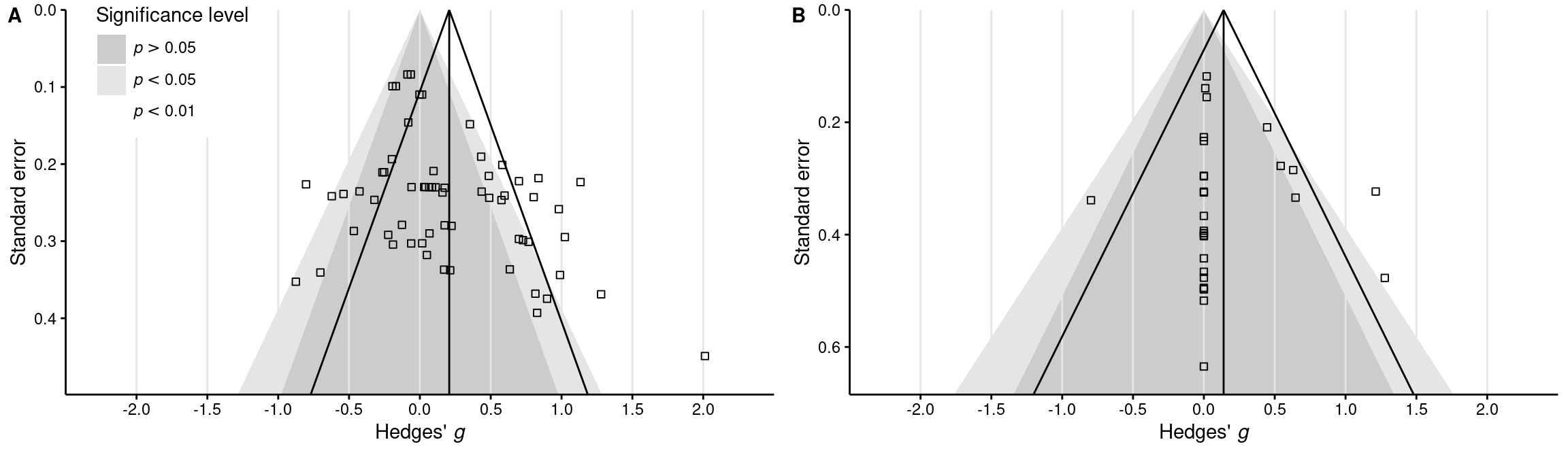
Egger regression test for mental rotation performance
Code
# Classical Egger regression test for the meta-analysis of rotation performance(egger_meta <-regtest(x = dat_meta$gi, sei = dat_meta$sei, model ="lm"))(egger_ci_meta <-confint(egger_meta$fit)["Xsei", ])
Regression Test for Funnel Plot Asymmetry

Model:     weighted regression with multiplicative dispersion
Predictor: standard error

Test for Funnel Plot Asymmetry: t = 3.4001, df = 60, p = 0.0012
Limit Estimate (as sei -> 0):   b = -0.2657 (CI: -0.4922, -0.0393)

    2.5 %    97.5 %
0.7958155 3.0702931
Egger regression test for gender differences
Code
# Classical Egger regression test for the meta-analysis of gender_differences(egger_gender <-regtest(x = dat_gender$gi, sei = dat_gender$sei, model ="lm"))(egger_ci_gender <-confint(egger_gender$fit)["Xsei", ])
Regression Test for Funnel Plot Asymmetry

Model:     weighted regression with multiplicative dispersion
Predictor: standard error

Test for Funnel Plot Asymmetry: t = 0.6481, df = 28, p = 0.5222
Limit Estimate (as sei -> 0):   b = 0.0319 (CI: -0.2452, 0.3091)

     2.5 %     97.5 %
-0.6879664  1.3247259
Funnel plot (Figure 4)
Code
# Create funnel plots for the two meta-analysesplots_funnel <-map2(list(dat_meta, dat_gender),list(summ_meta, summ_gender),function(dat, summ) {# Define maximul SE of interest (a bit larger than the largest observed SE) max_se <-max(dat$sei) +0.05# Compute a 95% funnel under the null hypothesis z_crit_05 <- stats::qnorm(0.975) funnel_greater_05 <-data.frame(x =c(0- z_crit_05 *sqrt(max_se^2), 0, 0+ z_crit_05 *sqrt(max_se^2)),y =c(max_se, 0, max_se),level ="greater_05" )# Compute a 99% funnel under the null hypothesis z_crit_01 <- stats::qnorm(0.995) funnel_smaller_05 <-data.frame(x =c(0- z_crit_01 *sqrt(max_se^2), 0, 0+ z_crit_01 *sqrt(max_se^2)),y =c(max_se, 0, max_se),level ="smaller_05" )# Create a third pseudo-funnel under the null hypothesis just for the legend funnel_smaller_01 <-mutate(funnel_greater_05, level ="smaller_01")# Compute a 95% funnel around the *observed* meta-analytic effect size funnel_observed <-mutate(funnel_greater_05, x = x + summ$intercept)# Plot the funnelsggplot(dat, aes(x = gi, y = sei)) +# Funnels under the null hypothesisgeom_polygon(data = funnel_smaller_01, aes(x = x, y = y, fill = level)) +geom_polygon(data = funnel_smaller_05, aes(x = x, y = y, fill = level)) +geom_polygon(data = funnel_greater_05, aes(x = x, y = y, fill = level)) +scale_fill_manual(values =c("gray80", "grey90", "white"),breaks =c("greater_05", "smaller_05", "smaller_01"),labels =c(expression(italic(p) >0.05),expression(italic(p) <0.05),expression(italic(p) <0.01) ) ) +# Grid linesgeom_vline(xintercept =seq(-2, 2, 0.5), color ="grey90") +# Observed_funnelgeom_path(data = funnel_observed, aes(x = x, y = y)) +# Meta-analytic effect sizegeom_vline(xintercept = summ$intercept, color ="black") +# Experiment-specific effect sizesgeom_point(shape =0) +# Stylingscale_x_continuous(breaks =seq(-2, 2, 0.5)) +scale_y_reverse() +coord_cartesian(xlim =c(-2.5, 2.5),ylim =c(max_se, 0),expand =FALSE ) +labs(x =expression("Hedges'"~italic("g")), y ="Standard error",fill ="Significance level" ) +theme_classic() +theme(axis.line =element_line(colour ="black"),axis.text =element_text(family ="Helvetica", color ="black"),axis.ticks =element_line(color ="black"),legend.position ="none",text =element_text(family ="Helvetica", color ="black") ) })# Extract legendlegend_funnel <-get_legend( plots_funnel[[1]] +theme(legend.position ="right"))# Combine plots and legendplot_grid(plotlist = plots_funnel, nrow =1, labels ="AUTO",label_size =11, label_fontfamily ="Helvetica") +draw_plot(legend_funnel, x =-0.39, y =0.355)# Save the plotggsave(here(figures_dir, "fig4_funnel.pdf"), width =12, height =3.5)# Save current workspacesave( run, data_dir, models_dir, figures_dir, tables_dir, n_iter, n_warmup, brms_file_refit, descriptives, dat_meta, dat_gender, res_meta, res_reg, res_gender, summ_gender, draws_gender, plots_funnel, legend_funnel,file =here("results", "workspace.RData"))
Source Code
# Main text## Setup```{r, message=FALSE}# Load packageslibrary(papaja)library(here)library(scales)library(tidyverse)library(furrr)library(metafor)library(brms)library(tidybayes)library(cowplot)# Load custom helper functionssource(here("misc", "helper_functions.R"))# Re-run steps that take a long time?run <-list(bayesian_models =FALSE,jackknife_analysis =FALSE,sensitivity_analysis =FALSE)# Options for MCMC sampling when fitting Bayesian multilevel modelsoptions(brms.backend ="cmdstanr") # Can choose "rstan" insteadoptions(mc.cores = parallel::detectCores()) # Use all available coresn_iter <-20000# Posterior samples per chain, including `n_warmup`n_warmup <-2000# Warmup samples per chainn_chains <-4# Number of (parallel) chainsseed <-1234# Random seed to make the results reproducible# Directory pathsdata_dir <-here("data")results_dir <-here("results")models_dir <-here(results_dir, "models")figures_dir <-here(results_dir, "figures")tables_dir <-here(results_dir, "tables")```## Introduction / Methods### Protocol#### PRISMA flowchart (Figure 1)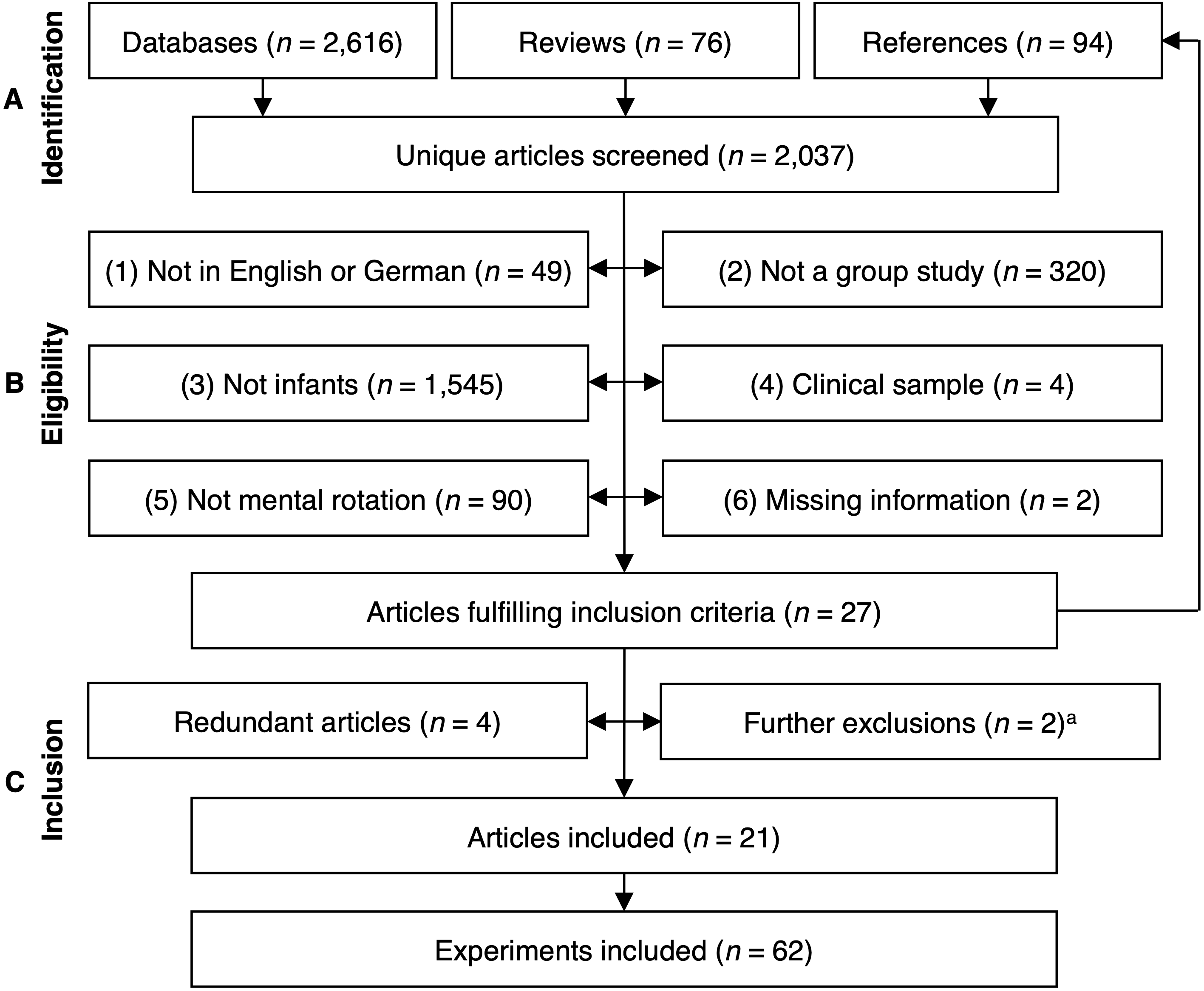### Selection process#### Percent agreement for binary decision (include vs. exclude)```{r}# Read the raw data from the screening processraw_screen <-read_tsv(here(data_dir, "02_screen.tsv"), na ="NA")# Percent agreement for binary decision (include vs. exclude)with(raw_screen, mean(bin_1 == bin_2))```#### Cohen's $\kappa_w$ (weighted kappa)```{r}# Cohen's kappawith(raw_screen, psych::cohen.kappa(cbind(bin_1, bin_2)))```#### Percent agreement for specific exclusion criteria```{r}# Compute interrater agreement for specific exclusion codeswith(raw_screen, mean(code_1 == code_2))```#### Cohen's $\kappa_w$ (weighted kappa)```{r}with(raw_screen, psych::cohen.kappa(cbind(code_1, code_2)))```### Effect measures#### Conversion of effect sizes for mental rotation performance```{r}# Read raw data for the meta-analysis of mental rotation performanceraw_meta <-read_tsv(here(data_dir, "03_meta.tsv"), na ="NA")# Add columns to the table of experimentsdat_all <- raw_meta %>%mutate(# Add unique experiment identifierexperiment =str_c(year, article, group, sep =", "),# Add difference between condition meansmean_diff =case_when(!is.na(mean_diff) ~ mean_diff,TRUE~ mean_novel - mean_familiar ),# Add d_z from paired-samples t-test of condition means (Rosenthal, 1991)d_z_t = t /sqrt(sample_size),# Add d_z from ANOVA F statistic via conversion to a t statisticd_z_f =sqrt(f) /sqrt(sample_size) * sign_f,# Add d_z from mean and standard deviation of the differenced_z_diff = mean_diff / sd_diff,# Add d_av from mean difference and standard deviations# See http://dx.doi.org/10.20982/tqmp.14.4.p242sd_av =sqrt((sd_novel^2+ sd_familiar^2) /2),d_av = mean_diff / sd_av,# Add d from one-sample t-test of novelty preference scoresd_nov_pref = (nov_pref -0.5) / sd_nov_pref,# Choose one type of outcome variable for each experimentdi =case_when(# 1. If d was reported directed!is.na(d) ~ d,# 2. If a paired-samples t-test was reported!is.na(d_z_t) ~ d_z_t,# 3. If an ANOVA was reported!is.na(d_z_f) ~ d_z_f,# 4. If the difference between means and its SD were reported!is.na(d_z_diff) ~ d_z_diff,# 5. If the individual condition means and their SDs were reported!is.na(d_av) ~ d_av,# 6. If a novelty preference score and its SD were reported!is.na(d_nov_pref) ~ d_nov_pref ),# Keep track which type of outcome measure was chosen for each articledi_type =case_when(!is.na(d) ~"d",!is.na(d_z_t) ~"d_z_t",!is.na(d_z_f) ~"d_z_f",!is.na(d_z_diff) ~"d_z_diff",!is.na(d_av) ~"d_av",!is.na(d_nov_pref) ~"d_nov_pref",TRUE~"none" ) %>%factor(levels =c("d", "d_z_t", "d_z_f", "d_z_diff", "d_av", "d_nov_pref", "none" )),# Apply small sample correction using Hedges' exact method# See http://dx.doi.org/10.20982/tqmp.14.4.p242dfi =2* (sample_size -1),ji =exp(lgamma(dfi /2) -log(sqrt(dfi /2)) -lgamma((dfi -1) /2)),gi = di * ji,# Recode gender as a categorical (factor) variable for meta-regressiongender =case_when( female_percent ==1.0~"Female", female_percent ==0.0~"Male",TRUE~"Mixed" ) %>%factor(levels =c("Mixed", "Female", "Male")),# Recode mean sample age in years (mean-centered) for meta-regressionage = age_mean /365.25,age_c = age -mean(age, na.rm =TRUE),# Recode task type as a categorical (factor) variable for meta-regressiontask =factor(task, levels =c("Habituation", "VoE")),# Combine gender and task into one column for plottinggender_task =factor(str_c(gender, task, sep =", "),levels =c("Female, Habituation","Male, Habituation","Mixed, Habituation","Mixed, VoE" ) ) ) %>%# Order rows by experiment IDarrange(experiment)# Compute standard errors of the effect sizes based on assumed correlation# See Hedges' formula on p. 253 in http://dx.doi.org/10.20982/tqmp.14.4.p242# You'll find a sensitivity analysis for `r_assumed` in the `supplement.Rmd`r_assumed <-0.5dat_meta_all <- dat_all %>%mutate(ni = sample_size,vi = (dfi / (dfi -2)) * ((2* (1- r_assumed)) / ni) * (1+ gi^2* (ni / (2* (1- r_assumed)))) - (gi^2/ ji^2),sei =sqrt(vi) ) %>%filter(!is.na(gi))# Extract either split or mixed experiments onlydat_split <-filter(dat_meta_all, gender_split %in%c("split", "split_only"))dat_mixed <-filter(dat_meta_all, gender_split %in%c("mixed", "mixed_only"))# Combine both strategies but preferring mixed experimentsdat_both_mixed <-filter( dat_meta_all, gender_split %in%c("mixed", "mixed_only", "split_only"))# Combine both strategies but preferring split experimentsdat_both_split <-filter( dat_meta_all, gender_split %in%c("split", "mixed_only", "split_only"))# We go ahead with the last solution (i.e., prefer split experiments) as to use# the maximum amount of information while not biasing the gender resultsdat_meta <- dat_both_split```#### Conversion of effect sizes for gender differences```{r}# Read raw data for the meta-analysis of gender differencesraw_gender <-read_tsv(here(data_dir, "04_gender.tsv"), na ="NA")# Compute relevant effect sizes for the meta-analysis of gender differencesdat_gender <- raw_gender %>%# Remove effect sizes from experiments with redundant samplesfilter(!redundant) %>%# Add columnsmutate(# Add unique experiment identifierexperiment =str_c(year, article, group, sep =", "),# Re-code non-significant F statistics as an effect size of d = 0f =as.numeric(f),f_assumed =ifelse(is.nan(f), 0, f),# Add d from two-samples t-test (Lakens, 2013)d_t = t *sqrt(1/ female_n +1/ male_n),# Add d from ANOVA F statistic via conversion to a t statisticd_f =sqrt(f_assumed) * sign_f *sqrt(1/ female_n +1/ male_n),# Add d from mean difference and pooled standard deviationmean_diff = mean_diff_males_mean - mean_diff_females_mean,sd_diff_pooled_numerator = (male_n -1) * (mean_diff_males_sd^2) + (female_n -1) * (mean_diff_females_sd^2),df = male_n + female_n -2,sd_diff_pooled =sqrt(sd_diff_pooled_numerator / df),d_diff = mean_diff / sd_diff_pooled,# Add d from one-sample t-test of novelty preference scoresmean_nov_pref = novelty_pref_males_mean - novelty_pref_females_mean,sd_nov_pref_pooled_numerator = (male_n -1) * (novelty_pref_males_sd^2) + (female_n) * (novelty_pref_females_sd^2),sd_nov_pref_pooled =sqrt(sd_nov_pref_pooled_numerator / df),d_nov_pref = mean_nov_pref / sd_nov_pref_pooled,# Choose one type of outcome variable for each experimentdi =case_when(# 1. If d was reported directed!is.na(d) ~ d,# 2. If a t-test was reported!is.na(d_t) ~ d_t,# 3. If an ANOVA was reported!is.na(d_f) ~ d_f,# 4. If the difference between means and their SDs were reported!is.na(d_diff) ~ d_diff,# 5. If novelty preference scores and their SDs were reported!is.na(d_nov_pref) ~ d_nov_pref ),# Keep track which type of outcome measure was chosen for each articledi_type =case_when(!is.na(d) ~"d",!is.na(d_t) ~"d_t",!is.na(d_f) ~"d_f",!is.na(d_diff) ~"d_diff",!is.na(d_nov_pref) ~"d_nov_pref" ) %>%factor(levels =c("d", "d_t", "d_f", "d_diff", "d_nov_pref")),# Apply small sample correction using Hedges' exact method# See http://dx.doi.org/10.20982/tqmp.14.4.p242j =exp(lgamma(df /2) -log(sqrt(df /2)) -lgamma((df -1) /2)),gi = di * j,# Compute standard error of Cohen's d, using harmonic mean of sample sizesni = female_n + male_n,nhi =2/ (1/ female_n +1/ male_n),vi = (df / (df -2)) * (2/ nhi) * (1+ gi^2* (nhi /2)) - (gi^2/ (j^2)),sei =sqrt(vi) ) %>%# Remove experiments that didn't provide any effect sizefilter(!is.na(gi))```#### Justification for excluding the Pedrett et al. (2020) paper```{r}# Justify exclusion of @pedrett2020 based on outlier mean agedescs_pedrett2020 <-list(age_years =2.56)within(descs_pedrett2020, { age_months <- age_years *12 next_largest_age_months <-max(dat_meta$age_mean) /30.417 age <- age_years *365.25 z <- (age -mean(dat_meta$age_mean)) /sd(dat_meta$age_mean)})```#### Descriptive information```{r}# Extract some descriptive statistics so we can paste them in the main text(descriptives <-list(n_articles =length(unique(dat_meta$article)),n_experiments =nrow(dat_meta),n_infants =sum(dat_meta$sample_size),percent_female =mean(dat_meta$female_percent, na.rm =TRUE),min_age_months =as.integer(min(dat_meta$age_min, na.rm =TRUE) /30.417),max_age_months =as.integer(max(dat_meta$age_max, na.rm =TRUE) /30.417),mean_age_weighted =print_days_months(sum(dat_meta$age_mean * dat_meta$ni) / (sum(dat_meta$ni)),long =TRUE ),n_experiments_habituation =nrow(filter(dat_meta, task =="Habituation")),n_experiments_voe =nrow(filter(dat_meta, task =="VoE"))))```#### Experiments included in the main analysis (Table 1)```{r}# Save table of experiments for the meta-analysis of rotationtab1 <- dat_meta %>%mutate(age_mean =print_days_months(age_mean),age_sd =str_c(as.character(round(age_sd)), "d"), ) %>%transmute(Article =if_else(article ==lag(article, default =""), "", article),Experiment = group,`Sample size`=as.integer(sample_size),Females =as.integer(round(female_percent * sample_size)),`Age ($M$ ± $SD$)`=ifelse(is.na(age_sd), paste(age_mean, "± n/a"), paste(age_mean, "±", age_sd) ),Task =as.character(task),`Stimulus type`=str_to_sentence(stimuli_presentation),`Stimulus dimensions`=str_c(as.integer(stimuli_dimensions), "D") ) %>%mutate(across(.fns =function(x) ifelse(is.na(x), "n/a", x)) )# Save the tabledir.create(tables_dir, showWarnings =FALSE)write_tsv(tab1, file =here(tables_dir, "tab1_experiments.tsv"), na ="n/a")# Add footnotescolnames(tab1)[5] <-str_c(colnames(tab1)[5], "^a^")tab1$Females[1] <-str_c(tab1$Females[1], "^b^")tab1$Task[3] <-str_c(tab1$Task[3], "^c^")# Display the tableapa_table( tab1,note =str_c("^a^ = mean ± standard deviation, ","^b^ = not available, ","^c^ = violation of expectation." ),landscape =TRUE, font_size ="scriptsize", escape =FALSE)```## Results### Mental rotation performance#### Prior predictive check```{r}# Specify priorsprior_meta <-c(set_prior("normal(0, 1)", class ="b"),set_prior("cauchy(0, 0.3)", class ="sd"))# Run prior predictive simulationdir.create(models_dir, showWarnings =FALSE, recursive =TRUE)brms_file_refit <-ifelse(run$bayesian_models, "always", "never")res_prior_meta <-brm( gi |se(sei) ~0+ Intercept + (1| article / experiment),data = dat_meta,prior = prior_meta,sample_prior ="only",save_pars =save_pars(all =TRUE),chains = n_chains,iter = n_iter,warmup = n_warmup,cores = n_chains,control =list(adapt_delta =0.99),seed = seed,file =here(models_dir, "res_prior_meta"),file_refit = brms_file_refit)summary(res_prior_meta)```#### Bayesian three-level meta-analysis```{r}# Run Bayesian multilevel modelres_meta <-update( res_prior_meta,sample_prior =FALSE,seed = seed,file =here(models_dir, "res_meta"),file_refit = brms_file_refit)summary(res_meta)```#### "Test" posterior probability mass above/below zero```{r}# Get posterior probability mass > 0 for the meta-analytic effecthypothesis(res_meta, "Intercept > 0")$hypothesis```#### Summary of model paramters incl. 95% credible interval (CrI)```{r}# Extract posterior draws for the meta-analytic effectsdraws_meta <-spread_draws( res_meta, `b_.*`, `sd_.*`,regex =TRUE, ndraws =NULL) %>%# Compute variances and ICC from standard deviationsmutate(intercept = b_Intercept,sigma_article = sd_article__Intercept,sigma_experiment =`sd_article:experiment__Intercept`,sigma2_article = sigma_article^2,sigma2_experiment = sigma_experiment^2,sigma2_total = sigma2_article + sigma2_experiment,icc = sigma2_article / sigma2_total,.keep ="unused" )# Summarize as means and 95% credible intervals(summ_meta <-mean_qi(draws_meta))```#### Forest plot (Figure 2)```{r, fig.height=14, fig.width=12}# Get posterior draws for the effect *in each experiment*epred_draws_meta <-epred_draws(res_meta, dat_meta, ndraws =NULL) %>%mutate(experiment_f =factor(experiment))# Create forest plotdir.create(figures_dir, showWarnings =FALSE)dat_meta %>%# Make sure the plot will be ordered alphabetically by experiment IDsarrange(experiment) %>%mutate(experiment_f =fct_rev(fct_expand(factor(experiment), "model")),# Show article labels only for the first experiment (row) per articlearticle =if_else(article ==lag(article, default =""), "", article),# Compute frequentist confidence intervals for each experimentci_lb = gi -qnorm(0.05/2, lower.tail =FALSE) *sqrt(vi),ci_ub = gi +qnorm(0.05/2, lower.tail =FALSE) *sqrt(vi),ci_print =print_mean_ci(gi, ci_lb, ci_ub) ) %>%# Prepare plotting canvasggplot(aes(x = gi, y = experiment_f)) +geom_vline(xintercept =seq(-3, 3, 0.5), color ="grey90") +# Add article and group labels as text on the leftgeom_text(aes(x =-9.9, label = article), hjust =0) +geom_text(aes(x =-7.1, label = group), hjust =0) +# Add experiment-specific effect sizes and CIs as text on the rightgeom_text(aes(x =3.7, label =print_num(gi)), hjust =1) +geom_text(aes(x =4.4, label =print_num(ci_lb)), hjust =1) +geom_text(aes(x =5.1, label =print_num(ci_ub)), hjust =1) +# Add Bayesian credible intervals for each experimentstat_interval(aes(x = .epred),data = epred_draws_meta,alpha = .8,point_interval ="mean_qi",.width =c(0.5, 0.95), ) +scale_color_grey(start =0.85, end =0.65,labels =as_mapper(~ scales::percent(as.numeric(.x))) ) +# Add experiment-specific effect sizes and CIs as dots with error barsgeom_linerange(aes(xmin = ci_lb, xmax = ci_ub), size =0.35) +geom_point(aes(size = ni), shape =22, fill ="white") +# Or (1 / vi)?# Add posterior distribution for the meta-analytic effectstat_halfeye(aes(x = intercept, y =-1), draws_meta,point_interval ="mean_qi",.width =c(0.95) ) +annotate("text",x =c(-9.9, 3.7, 4.4, 5.1),y =-0.5,label =c("Three-level model",print_num(summ_meta$intercept),print_num(summ_meta$intercept.lower),print_num(summ_meta$intercept.upper) ),hjust =c(0, 1, 1, 1),fontface ="bold" ) +# Add column headersannotate("rect",xmin =-Inf,xmax =Inf,ymin = descriptives$n_experiments +0.5,ymax =Inf,fill ="white" ) +annotate("text",x =c(-9.9, -7.1, 0, 3.7, 4.4, 5.1),y = descriptives$n_experiments +1.5,label =c("Article","Experiment","Effect size plot","Effect size","2.5%","97.5%" ),hjust =c(0, 0, 0.5, 1, 1, 1),fontface ="bold" ) +# Stylingcoord_cartesian(ylim =c(-1.5, descriptives$n_experiments +2), expand =FALSE,clip ="off" ) +scale_x_continuous(breaks =seq(-3, 3, 0.5)) +annotate("segment", x =-3.3, xend =3.3, y =-1.5, yend =-1.5) +labs(x =expression("Hedges'"~italic("g")),size ="Sample size",color ="CrI level" ) +theme_minimal() +theme(legend.position ="bottom",axis.text.x =element_text(family ="Helvetica", color ="black"),axis.text.y =element_blank(),axis.ticks.x =element_line(colour ="black"),axis.title.x =element_text(hjust =0.67, margin =margin(b =-15)),axis.title.y =element_blank(),panel.grid =element_blank(),text =element_text(family ="Helvetica") )# Save the plotdir.create(figures_dir, showWarnings =FALSE)ggsave(here(figures_dir, "fig2_meta.pdf"), width =12, height =14)```### Effects of gender, age, and task type#### Prior predictive check```{r}# Set numerical contrasts for factor variablescontrasts(dat_meta$gender) <- MASS::contr.sdif(3)contrasts(dat_meta$task) <- MASS::contr.sdif(2)# Specify priorsprior_reg <-c(set_prior("normal(0, 1)", class ="b", coef ="Intercept"),set_prior("normal(0, 0.5)", class ="b"),set_prior("cauchy(0, 0.3)", class ="sd"))# Run prior predictive simulationres_prior_reg <-brm( gi |se(sei) ~0+ Intercept + gender * age_c + task + (1| article / experiment),data = dat_meta,prior = prior_reg,sample_prior ="only",save_pars =save_pars(all =TRUE),chains = n_chains,iter = n_iter,warmup = n_warmup,cores = n_chains,control =list(adapt_delta =0.99),seed = seed,file =here(models_dir, "res_prior_reg"),file_refit = brms_file_refit)summary(res_prior_reg)```#### Bayesian three-level meta-regression```{r}# Run Bayesian multilevel modelres_reg <-update( res_prior_reg,sample_prior =FALSE,seed = seed,file =here(models_dir, "res_reg"),file_refit = brms_file_refit)summary(res_reg)```#### "Test" posterior probability mass above/below zero```{r}# Get posterior probability mass > 0 for all regression weightsbind_rows(hypothesis(res_reg, "Intercept > 0")$hypothesis,hypothesis(res_reg, "gender2M1 < 0")$hypothesis,hypothesis(res_reg, "gender3M2 > 0")$hypothesis,hypothesis(res_reg, "age_c > 0")$hypothesis,hypothesis(res_reg, "task2M1 > 0")$hypothesis,hypothesis(res_reg, "gender2M1:age_c > 0")$hypothesis,hypothesis(res_reg, "gender3M2:age_c > 0")$hypothesis)```#### Summary of model paramters incl. 95% CrI```{r}# Extract posterior draws for the meta-analytic effectsdraws_reg <-spread_draws( res_reg, `b_.*`, `sd_.*`,regex =TRUE, ndraws =NULL) %>%# Compute variances and ICC from standard deviationsmutate(intercept = b_Intercept,female_mixed = b_gender2M1,male_female = b_gender3M2,age = b_age_c,voe_habituation = b_task2M1,female_mixed_age =`b_gender2M1:age_c`,male_female_age =`b_gender3M2:age_c`,sigma_article = sd_article__Intercept,sigma_experiment =`sd_article:experiment__Intercept`,sigma2_article = sd_article__Intercept^2,sigma2_experiment =`sd_article:experiment__Intercept`^2,sigma2_total = sigma2_article + sigma2_experiment,icc = sigma2_article / sigma2_total, )# Summarize as means and 95% credible intervals(summ_reg <-mean_qi(draws_reg))```#### Meta-regression plot (Figure 3)```{r, fig.height=5, fig.width=12}# Get draws from the posterior distribution *for each experiment*epred_draws_reg <-epred_draws( res_reg, dat_meta,ndraws =NULL,re_formula =NA)# Use colors as proposed in https://arxiv.org/abs/2107.02270# The four colors code for a combination of tasks (Habituation, VoE) and gender# (female, male, mixed)plot_reg_colors <-list(habituation =c("Female, Habituation"="#5790fc","Male, Habituation"="#f89c20","Mixed, Habituation"="#e42536" ),voe =c("Mixed, VoE"="#964a8b"))# Create regression plotplot_reg <- dat_meta %>%ggplot(aes(x = age *12, y = gi)) +geom_hline(yintercept =seq(-1, 2, 0.5), color ="grey90") +annotate("rect",xmin =5.5, xmax =Inf, ymin =1.25, ymax =Inf,color =NA, fill ="white" ) +# Regression lines and CrIs for Habituation tasksstat_lineribbon(aes(y = .epred, color = gender_task),data = epred_draws_reg,alpha = .4,point_interval ="mean_qi",.width =c(0.5, 0.95) ) +# Individual study effect sizes for Habituation tasksgeom_point(aes(color = gender_task, size = ni), shape =0) +scale_color_manual(values = plot_reg_colors$habituation,breaks =names(plot_reg_colors$habituation),labels =c("Females", "Males", "Mixed gender"),na.value =NA ) +guides(color =guide_legend(title ="Habituation tasks",override.aes =list(fill =NA),order =1 )) +# Regression lines and CrIs for VoE tasks ggnewscale::new_scale_color() +stat_lineribbon(aes(y = .epred, color = gender_task),data = epred_draws_reg,fill =NA,alpha = .4,point_interval ="mean_qi",.width =c(0.5, 0.95) ) +# Individual study effect sizes for VoE tasksgeom_point(aes(color = gender_task, size = ni), shape =0) +scale_color_manual(values = plot_reg_colors$voe,breaks =names(plot_reg_colors$voe),labels =c("Mixed gender"),na.value =NA ) +guides(color =guide_legend(title ="VoE tasks", order =2)) +# Stylingcoord_cartesian(expand =FALSE) +scale_x_continuous(limits =c(2.9, 16.1), breaks =seq(3, 16, 1)) +scale_y_continuous(limits =c(-1.2, 2.2), breaks =seq(-1, 2, 0.5)) +scale_fill_grey(start =0.85, end =0.65,labels =as_mapper(~ scales::percent(as.numeric(.x))) ) +labs(x ="Age (months)",y =expression("Hedges'"~italic("g")),fill ="CrI level",size ="Sample size" ) +theme_classic() +theme(axis.text =element_text(family ="Helvetica", color ="black"),axis.ticks =element_line(color ="black"),legend.direction ="vertical",legend.key =element_blank(),legend.position ="none",panel.grid =element_blank(),text =element_text(family ="Helvetica", color ="black") )# Extract the legend so that we can put it inside the plot later onplot_reg_legend <-get_legend(plot_reg +theme(legend.position ="top"))# Define new labels for the regression coefficientscoef_colnames <-c(b_Intercept =expression("Intercept (Hedges'"~italic(g) *")"),b_gender2M1 =expression("Females - mixed"),b_gender3M2 =expression("Males - females"),b_age_c =expression("Age (per year)"),b_task2M1 =expression("Habituation - VoE"),`b_gender2M1:age_c`=expression("(Females - Mixed)"%*%"age"),`b_gender3M2:age_c`=expression("(Males - Females)"%*%"age"))# Plot posterior distributions of the regression coefficientsepred_draws_reg_coef <-tidy_draws(res_reg)plot_coef <- epred_draws_reg_coef %>%# Convert to long formatselect(all_of(names(coef_colnames))) %>%gather() %>%mutate(coef =factor(key, levels =names(coef_colnames))) %>%# Plot coefficients as "half eyes" (mean + CrIs + distribution)ggplot(aes(x = value, y =fct_rev(coef))) +geom_vline(xintercept =seq(-1, 1, 0.5), color ="grey90") +stat_halfeye(point_interval ="mean_qi", .width =c(0.5, 0.95)) +# Stylingcoord_cartesian(xlim =c(-1.25, 1.25), clip ="off") +scale_x_continuous(breaks =seq(-1, 1, 0.5)) +scale_y_discrete(labels = coef_colnames) +labs(x =expression("Regression weight ("* Delta *italic("g") *")")) +annotate("text",label ="Fixed effects", x =-3.175, y =7.86, hjust =0,family ="Helvetica", fontface ="bold", color ="black" ) +theme_minimal() +theme(axis.line.x =element_line(colour ="black"),axis.text.x =element_text(family ="Helvetica", color ="black"),axis.text.y =element_text(family ="Helvetica", color ="black", size =3.88* .pt,hjust =0, vjust =-0.1, margin =margin(l =20) ),axis.ticks.x =element_line(color ="black"),axis.ticks.y =element_blank(),axis.title.y =element_blank(),panel.grid =element_blank(),text =element_text(family ="Helvetica", color ="black") )# Combine the two regression plotsplot_grid( plot_reg, plot_coef,nrow =1, rel_widths =c(3, 2), labels ="AUTO",label_size =11, label_fontfamily ="Helvetica",label_x =0.008, label_y =0.99) +draw_plot(plot_reg_legend, x =0.385, y =0.865, hjust =0.5, vjust =0.5)# Save plotggsave(here(figures_dir, "fig3_reg.pdf"), width =12, height =5)```### Meta-analysis of gender differences#### Prior predictive check```{r}# Use the same priors as for the main meta-analysisprior_gender <- prior_meta# Run prior predictive simulationres_prior_gender <-brm( gi |se(sei) ~0+ Intercept + (1| article / experiment),data = dat_gender,prior = prior_gender,sample_prior ="only",save_pars =save_pars(all =TRUE),chains = n_chains,iter = n_iter,warmup = n_warmup,cores = n_chains,control =list(adapt_delta =0.99),seed = seed,file =here(models_dir, "res_prior_gender"),file_refit = brms_file_refit)summary(res_prior_gender)```#### Bayesian three-level meta-analysis```{r}# Run Bayesian multilevel modelres_gender <-update( res_prior_gender,sample_prior =FALSE,seed = seed,file =here(models_dir, "res_gender"),file_refit = brms_file_refit)summary(res_gender)```#### "Test" posterior probability mass above/below zero```{r}# Get posterior probability mass > 0 for the meta-analytic effecthypothesis(res_gender, "Intercept > 0")$hypothesis```#### Summary of model paramters incl. 95% CrI```{r}# Extract posterior draws for the meta-analytic effectsdraws_gender <-spread_draws( res_gender, `b_.*`, `sd_.*`,regex =TRUE, ndraws =NULL) %>%# Compute variances and ICC from standard deviationsmutate(intercept = b_Intercept,sigma_article = sd_article__Intercept,sigma_experiment =`sd_article:experiment__Intercept`,sigma2_article = sigma_article^2,sigma2_experiment = sigma_experiment^2,sigma2_total = sigma2_article + sigma2_experiment,icc = sigma2_article / sigma2_total,.keep ="unused" )# Summarize as means and 95% credible intervals(summ_gender <-mean_qi(draws_gender))```### Publication bias assessment#### Egger regression test for mental rotation performance```{r, echo=TRUE}# Classical Egger regression test for the meta-analysis of rotation performance(egger_meta <-regtest(x = dat_meta$gi, sei = dat_meta$sei, model ="lm"))(egger_ci_meta <-confint(egger_meta$fit)["Xsei", ])```#### Egger regression test for gender differences```{r}# Classical Egger regression test for the meta-analysis of gender_differences(egger_gender <-regtest(x = dat_gender$gi, sei = dat_gender$sei, model ="lm"))(egger_ci_gender <-confint(egger_gender$fit)["Xsei", ])```#### Funnel plot (Figure 4)```{r, fig.height=3.5, fig.width=12}# Create funnel plots for the two meta-analysesplots_funnel <-map2(list(dat_meta, dat_gender),list(summ_meta, summ_gender),function(dat, summ) {# Define maximul SE of interest (a bit larger than the largest observed SE) max_se <-max(dat$sei) +0.05# Compute a 95% funnel under the null hypothesis z_crit_05 <- stats::qnorm(0.975) funnel_greater_05 <-data.frame(x =c(0- z_crit_05 *sqrt(max_se^2), 0, 0+ z_crit_05 *sqrt(max_se^2)),y =c(max_se, 0, max_se),level ="greater_05" )# Compute a 99% funnel under the null hypothesis z_crit_01 <- stats::qnorm(0.995) funnel_smaller_05 <-data.frame(x =c(0- z_crit_01 *sqrt(max_se^2), 0, 0+ z_crit_01 *sqrt(max_se^2)),y =c(max_se, 0, max_se),level ="smaller_05" )# Create a third pseudo-funnel under the null hypothesis just for the legend funnel_smaller_01 <-mutate(funnel_greater_05, level ="smaller_01")# Compute a 95% funnel around the *observed* meta-analytic effect size funnel_observed <-mutate(funnel_greater_05, x = x + summ$intercept)# Plot the funnelsggplot(dat, aes(x = gi, y = sei)) +# Funnels under the null hypothesisgeom_polygon(data = funnel_smaller_01, aes(x = x, y = y, fill = level)) +geom_polygon(data = funnel_smaller_05, aes(x = x, y = y, fill = level)) +geom_polygon(data = funnel_greater_05, aes(x = x, y = y, fill = level)) +scale_fill_manual(values =c("gray80", "grey90", "white"),breaks =c("greater_05", "smaller_05", "smaller_01"),labels =c(expression(italic(p) >0.05),expression(italic(p) <0.05),expression(italic(p) <0.01) ) ) +# Grid linesgeom_vline(xintercept =seq(-2, 2, 0.5), color ="grey90") +# Observed_funnelgeom_path(data = funnel_observed, aes(x = x, y = y)) +# Meta-analytic effect sizegeom_vline(xintercept = summ$intercept, color ="black") +# Experiment-specific effect sizesgeom_point(shape =0) +# Stylingscale_x_continuous(breaks =seq(-2, 2, 0.5)) +scale_y_reverse() +coord_cartesian(xlim =c(-2.5, 2.5),ylim =c(max_se, 0),expand =FALSE ) +labs(x =expression("Hedges'"~italic("g")), y ="Standard error",fill ="Significance level" ) +theme_classic() +theme(axis.line =element_line(colour ="black"),axis.text =element_text(family ="Helvetica", color ="black"),axis.ticks =element_line(color ="black"),legend.position ="none",text =element_text(family ="Helvetica", color ="black") ) })# Extract legendlegend_funnel <-get_legend( plots_funnel[[1]] +theme(legend.position ="right"))# Combine plots and legendplot_grid(plotlist = plots_funnel, nrow =1, labels ="AUTO",label_size =11, label_fontfamily ="Helvetica") +draw_plot(legend_funnel, x =-0.39, y =0.355)# Save the plotggsave(here(figures_dir, "fig4_funnel.pdf"), width =12, height =3.5)# Save current workspacesave( run, data_dir, models_dir, figures_dir, tables_dir, n_iter, n_warmup, brms_file_refit, descriptives, dat_meta, dat_gender, res_meta, res_reg, res_gender, summ_gender, draws_gender, plots_funnel, legend_funnel,file =here("results", "workspace.RData"))```